Supervised Learning Problem

Supervised Learning Problem#

Prerequisites

Elements of Probability Theory
Define supervised and unsupervised learning
Give the difference between qualitative and quantitative variables and define of regression and classification

Learning Outcomes

Define a supervised learning problem

Example: Home Heating#

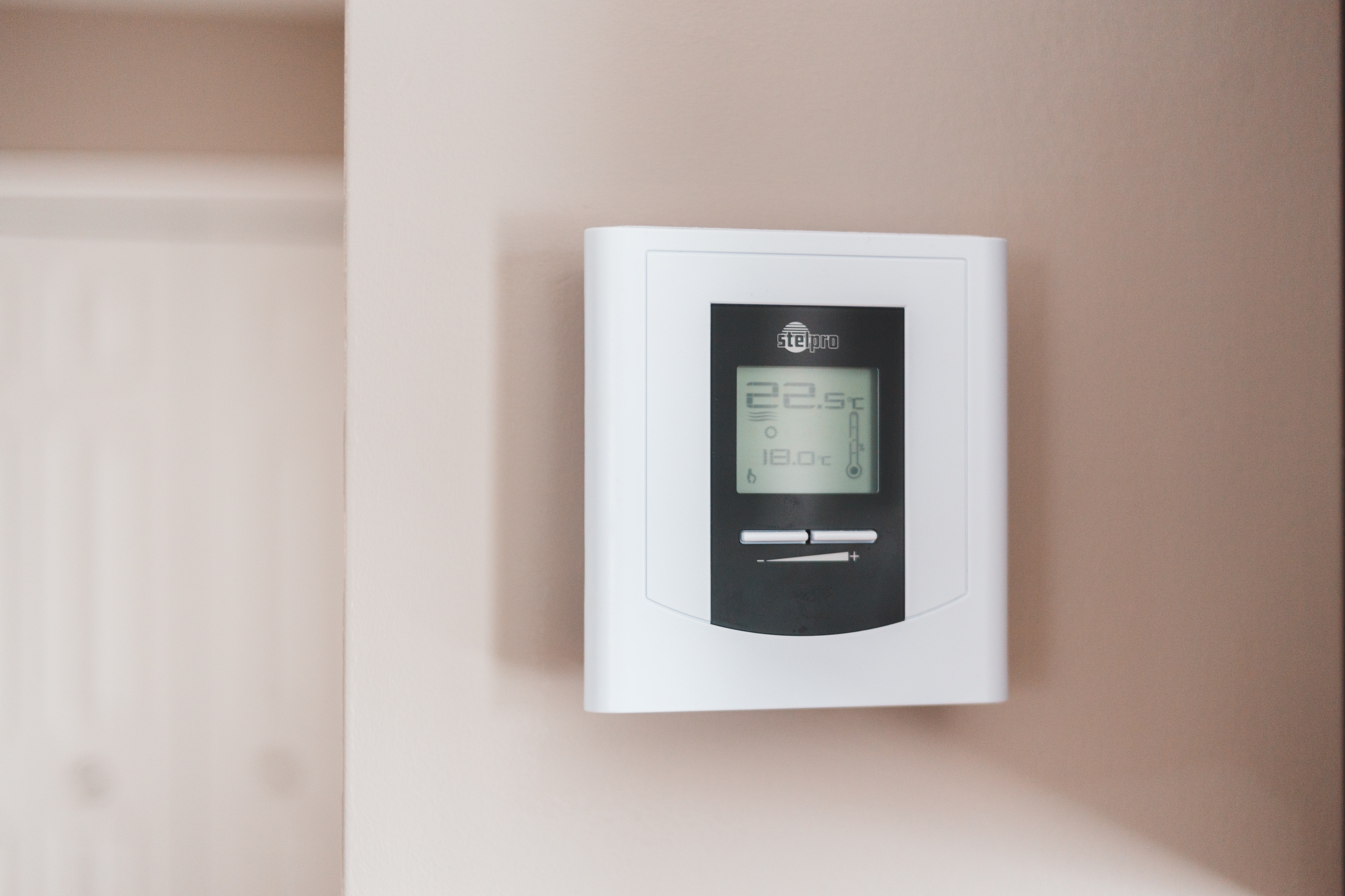
When its cold in my accommodation, I heat it.

\(\rightarrow\) I suspect a relationship between the energy I consume to heat my accommodation and the outdoor temperature, although other factors may also play a role.

How to predict how much energy I consume on average depending on the outdoor temperature ?

Three Different Approaches to Home-Heating Modeling#

Process-based	Expert-based	Statistical
Use some approximation of the heat equation in my accommodation given heat sources (radiators) and sinks (outdoor).	A thermal engineer diagnoses my accommodation based on his/her knowledge and/or on conventions.	Use energy-consumption and outdoor-temperature data to estimate parameters of a model.

Supervised Learning Objective#

To define a supervised-learning problem we need:

an input vector \(\boldsymbol{X}\) of \(X_1, \ldots, X_p\) input variables, or features and
an output or target variable \(Y\) used for supervision.

Supervised Learning Objective
Construct the “best” prediction rule to predict \(Y\) based on some training data: \((\boldsymbol{x}_i, y_i), i = 1, \ldots N\).

Supervised-Learning Flow: Fit and Predict#

Supervised-Learning Flow: Transform-Fit and Transform-Predict#

The \(i\)th observation of \(X_j\) in the sample is given by the element \(x_{ij}\) of the \(N\times p\) input-data matrix \(\mathbf{X}\).

The \(i\)th observation of \(y\) is given by the element \(y_i\) of the \(N \times 1\) output-data vector \(\mathbf{y}\).

Question

Recall the unbiased estimates of the sample mean \(\bar{y}\) and the sample variance \(s_Y^2\) of the random variable \(Y\) for some data \(y_i, 1 \le i \le N\).

Recall the unbiased estimate of the sample covariance \(q_{X, Y}\) between \(X\) and \(Y\) for \((x_i, y_i), 1 \le i \le N\).

Regression / Classification#

Regression	Classification
\(Y\) is quantitative	\(Y\) is qualitative

Example: Electricity Consumption Dependence on Temperature#

Raw input: temperature averaged over an administrative region of metropolitan France
Target: regional electricity consumption

Let’s first get familiar with the raw input data.

# Import modules
from pathlib import Path
import numpy as np
import pandas as pd
import holoviews as hv
hv.extension('bokeh')
import hvplot.pandas
import panel as pn

# Set data directory
data_dir = Path('data')

# Set keyword arguments for pd.read_csv
kwargs_read_csv = dict(header=0, index_col=0, parse_dates=True)

# Set first and last years
FIRST_YEAR = 2014
LAST_YEAR = 2021

# Define file path
filename = 'surface_temperature_merra2_{}-{}.csv'.format(
    FIRST_YEAR, LAST_YEAR)
filepath = Path(data_dir, filename)

# Read hourly temperature data averaged over each region
df_temp = pd.read_csv(filepath, **kwargs_read_csv).resample('D').mean()
temp_lim = [-5, 30]
label_temp = 'Temperature (°C)'

WIDTH = 260
# Scatter plot of demand versus temperature
def plot_temp(region_name, year):
    df = df_temp[[region_name]].loc[str(year)]
    df.columns = [label_temp]
    nt = df.shape[0]
    std = float(df.std(0))
    mean = pd.Series(df[label_temp].mean(), index=df.index)
    df_std = pd.DataFrame(
        {'low': mean - std, 'high': mean + std}, index=df.index)
    cdf = pd.DataFrame(index=df.sort_values(by=label_temp).values[:, 0],
                       data=(np.arange(nt)[:, None] + 1) / nt)
    cdf.index.name = label_temp
    cdf.columns = ['Probability']
    pts = df.hvplot(ylim=temp_lim, title='', width=WIDTH).opts(
        title='Time series, Mean, ± 1 STD') * hv.HLine(
        df[label_temp].mean()) * df_std.hvplot.area(
        y='low', y2='high', alpha=0.2)
    pcdf = cdf.hvplot(xlim=temp_lim, ylim=[0, 1], title='', width=WIDTH).opts(
        title='Cumulative Distrib. Func.') * hv.VLine(
        df[label_temp].mean())
    pkde = df.hvplot.kde(xlim=temp_lim,
                         width=WIDTH) * hv.VLine(
        df[label_temp].mean()).opts(title='Probability Density Func.')
    
    return pn.Row(pts, pcdf, pkde)

# Show
pn.interact(plot_temp, region_name=df_temp.columns,
            year=range(FIRST_YEAR, LAST_YEAR + 1))

/tmp/ipykernel_129/3467941216.py:7: FutureWarning: Calling float on a single element Series is deprecated and will raise a TypeError in the future. Use float(ser.iloc[0]) instead
  std = float(df.std(0))

Question

Describe how the mean and the standard deviation of the time series above depend on the region and on the year.

How do these dependencies show on the cumulative distribution and probability density functions?

Now let’s compare the target data with the input data.

# Read hourly demand data summed over each region
filename = 'reseaux_energies_demand_demand.csv'
filepath = Path(data_dir, filename)
df_dem = pd.read_csv(filepath, **kwargs_read_csv).resample('D').sum()
label_dem = 'Demand (MWh)'

# Scatter plot of demand versus temperature
def scatter_temp_dem(region_name, year):
    df = pd.concat([df_temp[region_name], df_dem[region_name]],
                   axis='columns', ignore_index=True).loc[str(year)]
    df.columns = [label_temp, label_dem]
    return df.hvplot.scatter(x=label_temp, y=label_dem, width=500,
                             xlim=[-5, 30])


text = pn.pane.Markdown("""
### Generalizing vs. Memorizing
#### New data will differ from training data.         
#### Plus there is *noise* from unresolved factors.      
#### -> we want to be able to *generalize*, not just *memorize*""")

# Show
pn.Row(pn.interact(scatter_temp_dem, region_name=df_dem.columns,
                   year=range(FIRST_YEAR, LAST_YEAR + 1)),
       pn.Spacer(width=20), text)

Supervised Learning Problem Definition#

Given the output \(Y\),

define features \(\boldsymbol{X} = (X_1, \ldots, X_p)\) based on (transformed) raw inputs
define model by a function \(f: \boldsymbol{X} \mapsto f(\boldsymbol{X})\)
define loss function \(L(Y, f(\boldsymbol{X}))\)
choose a training set \((\boldsymbol{x}_i, y_i), i = 1, \ldots, N\)

Example of model (linear): \(f_{\boldsymbol{\beta}}(\boldsymbol{X}) = \beta_0 + \sum_{j = 1}^p X_j \beta_j\)

Example of loss (squared error): \(L(Y, f(\boldsymbol{X})) = \left(Y - f(\boldsymbol{X})\right)^2\)

Assumption

All random variables and random vectors have finite variance and have densities (they are absolutely continuous with respect to the Lebesgue measure).

Expected Prediction Error
For some model function \(f\):

(23)#\[\begin{equation} \mathrm{EPE}(f) = \mathbb{E}(L(Y, f(\boldsymbol{X}))) = \int L(y, f(\boldsymbol{x})) \rho_{\boldsymbol{X}, Y}(\boldsymbol{x}, y) d\boldsymbol{x} dy, \end{equation}\]

where \(\rho_{\boldsymbol{X}, Y}\) is the joint probability density of \(\boldsymbol{X}\) and \(Y\).

Supervised Learning Objective (Concrete)
Find \(\hat{f}\) over all possible \(f\) such that the EPE is minimized.

Estimating the EPE#

If the law of large numbers applies and for a fixed number \(N\) of training data and an increasing number \(N' - N\) of new (test) data,

(24)#\[\begin{equation} \frac{1}{N'} \sum_{i = 1}^{N'} L(y_i, f(\boldsymbol{x}_i)) \underset{N' \to \infty}{\to} \mathrm{EPE}(f). \end{equation}\]

From the law of total expectation, we have that

(25)#\[\begin{align} \mathrm{EPE}(f) &= \mathbb{E}(\mathbb{E}[L(Y, f(X)) | X])\\ &= \int L(y, f(x)) \rho_{Y | X = x}(y) \rho_X(x)dy dx, \end{align}\]

where \(\rho_X\) is the probability density of \(X\) and \(\rho_{Y | X}\) is the conditional probability density of \(Y\) knowing \(X\).

The EPE can thus be interpreted as averaging over the inputs the prediction error for any input and can be minimized pointwise:

(26)#\[\begin{equation} f(x) = \mathrm{argmin}_c \mathbb{E}\left[L(Y, c) | X = x\right]. \end{equation}\]

Remark

Here, \(f\) is the best possible model among all possible functions of \(x\).

This is a theoretical notion.

In practice, we look for an \(f\) in a set of models which is smaller than the set of all possible functions of \(x\) (e.g. a linear model).

In that case, the model must be trained over all points in a relatively large sample so that the minimization cannot in general be done pointwise.

The Case of Squared Error Loss#

The EPE using the squared error loss is

(27)#\[\begin{equation} \mathrm{EPE}(f) = \mathbb{E}((Y - f(X))^2). \end{equation}\]

Then

(28)#\[\begin{equation} f(x) = \underset{c}{\mathrm{argmin}} \ \mathbb{E}\left[(Y - c)^2 | X = x\right]. \end{equation}\]

Since the expectation is the value that minimizes the expectation of the squared deviations (see Appendix: Elements of Probability Theory), the optimal solution is

(29)#\[\begin{equation} f(x) = \mathbb{E}(Y | X = x) \end{equation}\]

In other words:

Theorem

The best prediction of the output for any input is the conditional expectation, when best is measured by the average squared error and the optimum is looked for over all possible functions of \(x\).

Question (optional)

What is the statistic giving the solution minimizing the EPE if we use the absolute error loss \(|Y - f(X)|\) instead of the squared error loss?