Classification II: Discriminative models

Classification II: Discriminative models#

Prerequisites

Generative models
Vector and matrix derivative

Learning Outcomes

Define a discriminative model.
Apply a logistic regression.
Perform a Fisher Linear discriminant analysis (F-LDA) for dimension reduction.

Case study: Rain prediction#

We apply the following methods to the prediction of whether it rains (\(C = 1\)) or not (\(C = 0\)) from climate variables, as in the notebook Classification I: Generative models.

# Import data analysis modules
import matplotlib.pyplot as plt
import numpy as np
import pandas as pd
plt.rc('font', size=14)
RC_COLORS = [d['color'] for d in plt.rcParams['axes.prop_cycle']]

# Load data
df = pd.read_csv("data/era5_paris_sf_2000_2009.csv",
                 index_col='time', parse_dates=True)

# Normalize the variables
df_norm = (df - df.mean()) /df.std()

# Select variables and resample to daily values
df_day = df_norm[['tp', 'sp', 't2m']].resample("D").mean()

# Assign tag to precipitation
PRECIP_TH = -0.2 # normalized threshold
df_day['tag'] = df_day['tp'].where(df_day['tp'] > PRECIP_TH, 0)
df_day['tag'] = df_day['tag'].where(df_day['tp'] <= PRECIP_TH, 1)

Discriminative models#

In the notebook Classification I: Generative models, the Bayes’ theorem is applied to invert the classification problem: the focus is on class densities \(\boldsymbol x \mapsto f_{\boldsymbol X|C}(\boldsymbol x | k)\) or the likelihood functions \(k \mapsto f_{\boldsymbol X|C}(\boldsymbol x | k)\).

Here, we instead directly estimate the probability \(P(C = k | \boldsymbol X = \boldsymbol x)\) to observe a class \(k\) given an input \(\boldsymbol x\).

If we know this probability for all classes, we can then assign an observation to the class that has the maximum probability according to the Bayes classifier.

Discriminative models based on regression#

We first consider to classification models that are based on regression:

linear regression and
logistic regression.

Both are linear models (in the generalized sense).

Two-classes problem#

Let us consider a simple problem with only 2 classes: \(C = 0\) or 1. We must have,

\[ P(C = 0 | \boldsymbol X = \boldsymbol x) = 1 - P(C = 1 | \boldsymbol X = \boldsymbol x).\]

Thus, setting \(y(\boldsymbol x) = P(C = 1 | \boldsymbol X = \boldsymbol x)\), we can assign a real number to the probability of the class \(C = 1\) for each input.

We can then apply the indicator function \(I_{(0.5, +\infty)}(y) = 1\) if \(y > 0.5\), 0 otherwise, to assign points to the two classes.

The classification problem thus translates into a regression problem.

Linear regression for classification#

In linear regression for classification, the regression method is that of the Ordinary Least Square (OLS) applied to a target given by the indicator response, i.e. such that \(y = 1\) if \(k = 1\) else 0.

The decision boundary is the set of \(\boldsymbol x\) such that \(y(\boldsymbol x) = \beta_0 + \boldsymbol \beta^\top \boldsymbol x = 0.5\).

For \(p = 1\), the decision point is given by \(x = (0.5 - \beta) / \alpha\).

The figure below illustrates this approach for our case study.

Warning

Here, \(y\) does not represent some quantity of rain, but the probability that it rains.

# Import the linear regression class
from sklearn.linear_model import LinearRegression

# Fit linear regression model
ols = LinearRegression()
_ = ols.fit(df_day[['sp']], df_day['tag'])

# Get decision boundary
boundary = (.5 - ols.intercept_) / ols.coef_[0]

# Plot targets and predictions
fig, ax = plt.subplots()
sp_test = np.linspace(-4, 3, 300)
ax.plot(sp_test, ols.coef_ * sp_test + ols.intercept_, 'r',
        label="OLS prediction")
ax.axvline(boundary, linestyle='--', color='.5',
           label="Decision boundary")
ax.scatter(df_day['sp'], df_day['tag'], s=4, alpha=0.1,
           label="Target")
ax.set_xlabel('x: Normalized pressure')
ax.set_ylabel('y: Rain tag')
ax.set_xlim(-4, 3.)
ax.set_ylim(-0.5, 2.)
ax2 = ax.twiny()
ax2.set_xlim(ax.get_xlim())
ax2.set_xticks([boundary.round(2)])
_ = ax.legend(loc='upper left')

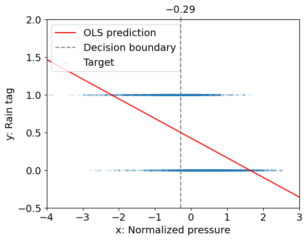
../_images/8549a11947833cb6fc1467a661c8a9e171dd7ea3d51d3dbb49bbdfab1040d200.png

Interpretation:

The fit that we obtain is not too bad: there seem to be a tendency for low pressure days to be rainy and high pressure days to be dry, with a decision boundary given by \(x \approx -0.29\).
This is not fully satisfactory however because \(y(x)\) is not restricted to take values between 0 and 1 and so \(y\) is not a probability.

Warning

For \(K = 2\), linear regression of the indicator response(s) provides coefficients that correspond to those of linear discriminant analysis but for the intercept (Chap. 4 in Hastie et al. 2009).
Linear regression for classification easily generalizes to multiple classes. However, for \(K > 2\), classes can be masked by others due to the rigid nature of the linear regression model (Chap. 4 in Hastie et al. 2009).

Logistic regression#

Logistic regression for two classes and one input#

In order to address the above problem, we are going to fit a non-linear function of \(x\) called the sigmoid:

(59)#\[\begin{equation} y(x) = \frac{1}{1 + e^{-x}} \end{equation}\]

Question

Check that for any \(x\), \(0 < y(x) < 1\).

For which value of \(x\) do we have \(y(x) = 0.5\).

Introduce a parameter in the function in order to control that threshold.

Introduce a second parameter to control the speed of the transition from \(y\simeq 0\) to \(y\simeq 1\).

Hence, \(y(x)\) can be interpreted as a probability conditioned on the observation \(x\).
In order to adjust this conditional probability, we introduce the parameters \(\beta_0\) and \(\beta_1\) and maximize the probability \(y(\beta_0 + \beta_1 x)\), so that the decision boundary is at \(x = -\beta_0 / \beta_1\).
Because this function is non-linear, we no longer have an analytical solution and we instead need a non-linear solver to find \(\beta_0\) and \(\beta_1\).

Below is an example for the same data set as above using the linear_model.LogisticRegression model implemented in Scikit-Learn.

# Import the logistic regression class
from sklearn.linear_model import LogisticRegression

# Define sigmoid function
def sigmoid(x):                                        
    return 1 / (1 + np.exp(-x))

# Fit logistic regression model using scikit-learn
clf = LogisticRegression()
clf.fit(df_day[['sp']], df_day['tag'])

# Get decision boundary
boundary = -clf.intercept_[0] / clf.coef_[0, 0]

# Plot target and predictions
fig, ax = plt.subplots()
loss = sigmoid(sp_test * clf.coef_[0, :] + clf.intercept_)
ax.plot(sp_test, loss, color='red', label="Logistic prediction")
ax.axvline(boundary, linestyle='--', color='.5',
           label="Decision boundary")
ax.scatter(df_day['sp'], df_day['tag'], s=4, alpha=0.1,
           label="Target")
ax.set_xlabel('x: Normalized pressure')
ax.set_ylabel('y: Rain tag')
ax.set_xlim(-4, 3.)
ax.set_ylim(-0.5, 2.)
ax2 = ax.twiny()
ax2.set_xlim(ax.get_xlim())
ax2.set_xticks([boundary.round(2)])
_ = ax.legend(loc='upper left')

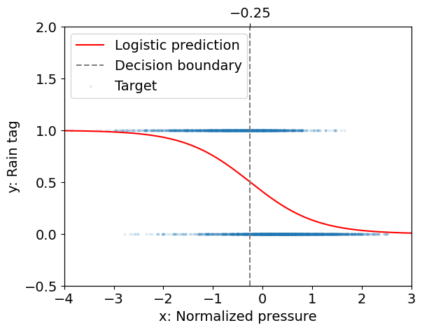
../_images/affb5d844f7750034603b88c0f517eed650d5c205e262702e30097e3e3c2c6a9.png

Interpretation:

The decision boundary for logistic regression (\(x \approx -0.25\)) is close to that for linear regression (\(x \approx -0.29\)).
However we can now assign an estimate of the probability for the “rain” event given an observation of the pressure.
That probability depends on the distance of the observed pressure to the pressure at the decision boundary, i.e. on both \(\beta_0\) and \(\beta_1\), while its rate of change with the input is controled by \(\beta_1\).

Note that the sigmoid function has many interesting properties. For instance we can invert this function to get

(60)#\[\begin{equation} x = \ln\frac{y}{1 -y} \end{equation}\]

where \(x\) is now the logarithm of the odds. This function \(x(y)\) is called the logit function.

Another property is that the derivative of the sigmoid is easy to compute:

(61)#\[\begin{equation} \frac{dy}{dx} = y(1-y) \end{equation}\]

We will use this property when we will study neural networks.

Generalization to multiple classes and inputs#

The example above is relatively straightforward because there are only two classes.
We took advantage of this when we identified the class identifier with the probability of one of the two classes given the input.
We can no longer do that when we consider more than two classes.

In the multiple class problem the logistic function can be generalized to,

(62)#\[\begin{equation} P(C = k | \boldsymbol X = \boldsymbol x) := y_k(\boldsymbol x) = \frac{\exp(\beta_{k 0} + \boldsymbol \beta_k^\top \boldsymbol x) }{\sum_{l = 1}^{K - 1} \exp (\beta_{l0} + \boldsymbol \beta_l^\top \boldsymbol x)}, \end{equation}\]

where \(\beta_{k0}\) in \(\mathbb{R}\) and \(\boldsymbol \beta_k\) in \(\mathbb{R}^p\) for \(1 \le k \le K - 1\).

As before we can use a non linear solver to find the numerical values of the \(\beta_{k0}\) and \(\boldsymbol \beta_k\).

Link to Linear Discriminant Analysis (LDA)#

In the case of LDA (Classification I: Generative models), the log-posterior odds between class \(k\) and \(K\) are linear functions of \(\boldsymbol x\):

\[\begin{split} \begin{aligned} \log \frac{P(C = k | \boldsymbol X = \boldsymbol x)}{P(C = K | \boldsymbol X = \boldsymbol x)} &= - \frac{1}{2} (\boldsymbol \mu_k + \boldsymbol \mu_K)^\top \boldsymbol \Sigma^{-1} (\boldsymbol \mu_k - \boldsymbol \mu_K) \\ &+\log \frac{P_k}{P_K} + (\boldsymbol \mu_k - \boldsymbol \mu_K)^\top \boldsymbol \Sigma^{-1} \boldsymbol x \\ &= \alpha_{k 0} + \boldsymbol \alpha_{k}^\top \boldsymbol x \end{aligned} \end{split}\]

This linearity is a consequence of the Gaussian assumption for the class densities, as well as the assumption of a common covariance matrix.

The linear logistic model by construction has linear logits:

\[ \begin{aligned} \log \frac{P(C = k | \boldsymbol X = \boldsymbol x)}{P(C = K | \boldsymbol X = \boldsymbol x)} &= \beta_{k 0} + \boldsymbol \beta_{k}^\top \boldsymbol x \end{aligned} \]

It seems that the models are the same.
However, LDA assumes that \(P(\boldsymbol X = \boldsymbol x)\) is a Gaussian mixture, while we can think of it as being estimated in a fully nonparametric and unrestricted fashion in logistic regression.
It is generally felt that logistic regression is a safer, more robust bet than the LDA model, relying on fewer assumptions, even though results may be similar in practice (Chap. 4 in Hastie et al. 2009).

Conclusion on logistic regression#

Logistic regression is a powerful strategy that does not make any assumption about the distribution of the data in the input space.
It provides a probability of belonging to a class given an input.
The major drawback of the logistic regression is that, by design, we suppose that there is a linear relationship between the log odds of the output variable and the input variables.
This is problematic of course when this relation does not hold in which case nonlinear models may be needed.

Optimal dimension reduction for classification: Fisher Linear Discriminant Analysis#

So far, we have not considered problems with a high number of features.
However, the feature space is often high-dimensional, thus prohibiting visualizing the classes and making overfitting more likely.
Fisher Linear Discriminant Analysis (F-LDA) is a method to tackle this problem: it relies on projecting the data set onto a reduced number of dimensions that are best suited to separate the classes.
(Another other popular tool for dimension reduction is Principal Component Analysis, see Introduction to Unsupervised Learning with a Focus on PCA.)

To present this method, let us use a 2-dimensional dataset \((\boldsymbol x_i, k_i), 1 \le i \le N\) with two classes \(C = 0\) and \(C = 1\) (e.g. pressure and temperature and no rain/rain).

CLASS_LABELS = [r'$C = 0$', r'$C = 1$']
DIM_LABELS = [r'$x_1$', r'$x_2$']

N = 1000
THETA = np.pi / 6
MU_1 = np.array([-10, 0])
MU_2 = np.array([10, 0])
SIGMA_V = np.array([10, 1])

Rw = np.array([[np.cos(THETA), -np.sin(THETA)],
               [np.sin(THETA), np.cos(THETA)]])
Cv = np.diag(SIGMA_V**2)
Cw = Rw @ Cv @ Rw.T

z1 = np.random.multivariate_normal(MU_1, Cw, N)
z2 = np.random.multivariate_normal(MU_2, Cw, N)

fig, ax = plt.subplots(1)
s = 2
alpha_scatter = 0.2
ax.scatter(z1[:, 0], z1[:, 1], s=s, alpha=alpha_scatter,
           label=CLASS_LABELS[0])
ax.scatter(z2[:, 0], z2[:, 1], s=s, alpha=alpha_scatter,
           label=CLASS_LABELS[1])
ax.set_xlabel(DIM_LABELS[0])
ax.set_ylabel(DIM_LABELS[1])
_ = ax.legend()

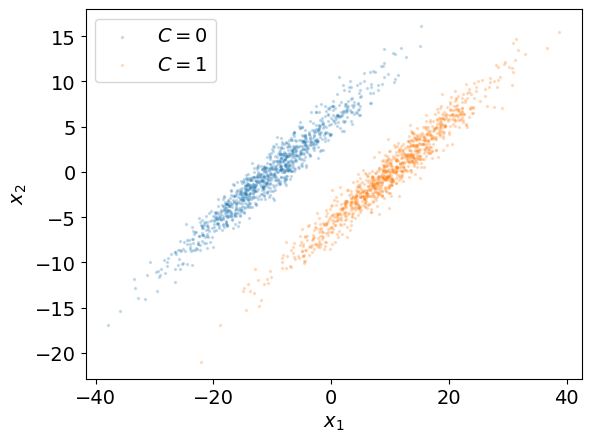
../_images/3b26235f0dbd2ba90cbcb240bbe6df7e8a6dcb18cce7e84ec224e5e2a0ca61c5.png

In the example above, we have observations from two distinct and well separated classes: a boundary separating these classes can be drawn.

The plots below represent the histograms of the data along the dimensions \(x_1\) and \(x_2\) in order to study whether or not the classes can be separated in each of these dimensions.

ztot = np.concatenate((z1, z2), 0)

alpha_hist = 0.3
density = True
bins = 20

fig, ax = plt.subplots(1, 2, sharey=True, figsize=(10, 4))
ax[0].hist(z1[:, 0], bins, density=density, alpha=alpha_hist,
           label=CLASS_LABELS[0])
ax[0].hist(z2[:, 0], bins, density=density, alpha=alpha_hist,
           label=CLASS_LABELS[1])
ax[0].set_xlabel(DIM_LABELS[0])
ax[0].legend()

ax[1].hist(z1[:, 1], bins, density=density, alpha=alpha_hist,
           label=CLASS_LABELS[0])
ax[1].hist(z2[:, 1], bins, density=density, alpha=alpha_hist,
           label=CLASS_LABELS[1])
ax[1].set_xlabel(DIM_LABELS[1])
_ = ax[1].legend()

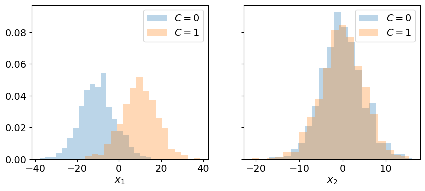
../_images/7b005ba64c9ebe13c569f439f7983ee2a837ec8d7a632fccfeafb0f0aa6c46fa.png

Interpretation:

The projection of the data from the original parameter space \((x_1, x_2)\) to each dimension mixes the two classes: they can no longer be separated by a boundary.

Problem:

Can we find a vector given by the linear combination of \(\boldsymbol e_1\) and \(\boldsymbol e_2\) so that the two classes are best separated for the data projected on this vector?

We look for a vector \(\boldsymbol \beta\) that best discriminate between the two classes.

Given \(\boldsymbol \beta\), the projection of an input vector on this vector is given by

(63)#\[\begin{equation} z = \boldsymbol \beta^\top \boldsymbol x. \end{equation}\]

We can then propose a threshold \(z_0\) such that if \(z > z_0\) we assign a point to class \(C = 0\) and if \( z \le z_0\) we assign this point to \(C = 1\).

Question

In the example above, do you have an idea of which axis you could use to project the data and get maximum class separability?

A first attempt: maximizing the distance between the conditional means#

In order to find a direction that best separates each class, a first approach could to maximize the distance between the sample means of the input data for each class.

In the original coordinate system, these means are given by,

(64)#\[\begin{equation} \begin{aligned} \hat{\boldsymbol \mu}_0 &= \frac{1}{N_0} \sum_{i, k_i = 0} \boldsymbol x_i\\ \hat{\boldsymbol \mu}_1 &= \frac{1}{N_1} \sum_{i, k_i = 1} \boldsymbol x_i. \end{aligned} \end{equation}\]

The projection of these means onto the vector \(\boldsymbol \beta\) is given by,

(65)#\[\begin{equation} \begin{aligned} \nu_0^{\boldsymbol \beta} &= \boldsymbol \beta^\top \hat{\boldsymbol \mu}_0\\ \nu_1^{\boldsymbol \beta} &= \boldsymbol \beta^\top \hat{\boldsymbol \mu}_1 . \end{aligned} \end{equation}\]

Objective: Find the vector \(\boldsymbol \beta\) that maximizes

(66)#\[\begin{equation} J(\boldsymbol \beta) = \left(\nu_1^{\boldsymbol \beta} - \nu_0^{\boldsymbol \beta}\right)^2. \end{equation}\]

Question (optional)

Show that

(67)#\[\begin{equation} \left(\nu_1^{\boldsymbol \beta} - \nu_0^{\boldsymbol \beta}\right)^2 = \boldsymbol \beta^\top \boldsymbol S_b \boldsymbol \beta, \end{equation}\]

with

(68)#\[\begin{equation} \boldsymbol S_b := \left(\hat{\boldsymbol\mu}_1^{\boldsymbol \beta} - \hat{\boldsymbol\mu}_0^{\boldsymbol \beta}\right) \left(\hat{\boldsymbol\mu}_1^{\boldsymbol \beta} - \hat{\boldsymbol\mu}_0^{\boldsymbol \beta}\right)^\top, \end{equation}\]

the between class scatter matrix.

The cost function can be arbitrarily big if we take \(\boldsymbol \beta\) as big as we want.

In order to find the direction \(\boldsymbol \beta\), we need to add a constraint on the norm \(\lVert \boldsymbol \beta \lVert\) to the cost function.

The new cost function is,

(69)#\[\begin{equation} J(\boldsymbol \beta) = \left(\hat{\nu}_1^{\boldsymbol \beta} - \hat{\nu}_0^{\boldsymbol \beta}\right)^2 - \lambda (\boldsymbol \beta^\top \boldsymbol \beta - 1), \end{equation}\]

with \(\lambda \ge 0\) a Lagrange multiplier.

Question (optional)

Differentiate the cost function \(J(\boldsymbol \beta)\) with respect to \(\boldsymbol \beta\) and show that \(\nabla J = 0\) when

(70)#\[\begin{equation} \boldsymbol S_b \boldsymbol \beta = \lambda \boldsymbol \beta, \end{equation}\]

for some \(\lambda \ge 0\).

However,

(71)#\[\begin{equation} \begin{aligned} \boldsymbol S_b \boldsymbol \beta &= \left(\hat{\boldsymbol\mu}_1^{\boldsymbol \beta} - \hat{\boldsymbol\mu}_0^{\boldsymbol \beta}\right) \left[\left(\hat{\boldsymbol\mu}_1^{\boldsymbol \beta} - \hat{\boldsymbol\mu}_0^{\boldsymbol \beta}\right)^\top \boldsymbol \beta\right] \\ & \propto \left(\hat{\boldsymbol\mu}_1^{\boldsymbol \beta} - \hat{\boldsymbol\mu}_0^{\boldsymbol \beta}\right). \end{aligned} \end{equation}\]

In other words, \(\boldsymbol S_b\) is a matrix that projects on \(\hat{\boldsymbol\mu}_1^{\boldsymbol \beta} - \hat{\boldsymbol\mu}_0^{\boldsymbol \beta}\).

Thus, \(J\) is maximum when

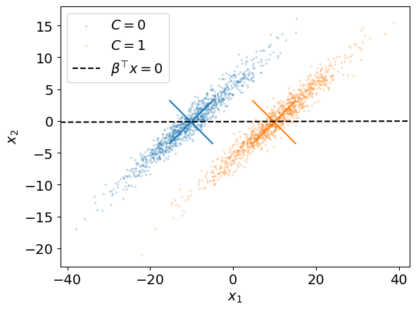
(72)#\[\begin{equation} \boldsymbol \beta \propto \left(\hat{\boldsymbol\mu}_1^{\boldsymbol \beta} - \hat{\boldsymbol\mu}_0^{\boldsymbol \beta}\right). \end{equation}\]

That is \(\boldsymbol \beta\) is the direction that joins the two sample means.

Unfortunately, this does not necessarily ensures that the classes are well separated when projected onto \(\boldsymbol \beta\).

For instance, the line spanned by this vector is represented below for our example.

mu_0_hat = z1.mean(0)
mu_1_hat = z2.mean(0)
beta = (mu_1_hat - mu_0_hat)

fig, ax = plt.subplots(1)
s_mu = s * 1000
marker_mu = 'x'
ax.scatter(z1[:, 0], z1[:, 1], s=s, alpha=alpha_scatter,
           label=CLASS_LABELS[0])
ax.scatter(z2[:, 0], z2[:, 1], s=s, alpha=alpha_scatter,
           label=CLASS_LABELS[1])
ax.scatter(*mu_0_hat, s=s_mu, marker=marker_mu, c=RC_COLORS[0])
ax.scatter(*mu_1_hat, s=s_mu, marker=marker_mu, c=RC_COLORS[1])
xlim = ax.get_xlim()
ylim = ax.get_ylim()
x = np.linspace(*xlim, 1000)
y_line = mu_0_hat[1] + beta[1] / beta[0] * (x - mu_0_hat[0])
ax.plot(x, y_line, '--k', label=r'$\beta^\top x = 0$')
ax.set_xlim(xlim)
ax.set_ylim(ylim)
ax.set_xlabel(DIM_LABELS[0])
ax.set_ylabel(DIM_LABELS[1])
_ = plt.legend()

../_images/d3f97a8a233a81ffadc8775728b95f787ee4f2487ef86b7d4ddeabf999efdc36.png

Second attempt: maximizing the means relatively to the variances#

We introduce for each class a quantity that is proportional to the sample variance of the data projected on \(\beta\):

(73)#\[\begin{equation} \begin{aligned} \left(s_0^{\boldsymbol \beta}\right)^2 &= \sum_{i, k_i = 0} \left(\boldsymbol \beta^\top \boldsymbol x_i - \nu_0^{\boldsymbol \beta}\right)^2\\ \left(s_1^{\boldsymbol \beta}\right)^2 &= \sum_{i, k_i = 1} \left(\boldsymbol \beta^\top \boldsymbol x_i - \nu_1^{\boldsymbol \beta}\right)^2, \end{aligned} \end{equation}\]

Then, we want \((s_0^{\boldsymbol \beta})^2 + (s_1^{\boldsymbol \beta})^2\) to be as small as possible.

In a similar way as before, we can show that

(74)#\[\begin{equation} \left(s_0^{\boldsymbol \beta}\right)^2 + \left(s_1^{\boldsymbol \beta}\right)^2 = \boldsymbol \beta^\top \boldsymbol S_w \boldsymbol \beta \end{equation}\]

with \(\boldsymbol S_w\) the within class scatter matrix,

(75)#\[\begin{equation} \boldsymbol S_w := \sum_{i, k_i = 0} (\boldsymbol x_i - \hat{\boldsymbol\mu}_0^{\boldsymbol \beta}) (\boldsymbol x_i - \hat{\boldsymbol\mu}_0^{\boldsymbol \beta})^\top + \sum_{i, k_i = 1} (\boldsymbol x_i - \hat{\boldsymbol\mu}_1^{\boldsymbol \beta}) (\boldsymbol x_i - \hat{\boldsymbol\mu}_1^{\boldsymbol \beta})^\top. \end{equation}\]

We define a new cost function that combines these two metrics:

(76)#\[\begin{equation} J(\mathbf w) = \frac{\left(\hat{\nu}_1^{\boldsymbol \beta} - \hat{\nu}_0^{\boldsymbol \beta}\right)^2}{\left(s_0^{\boldsymbol \beta}\right)^2 + \left(s_1^{\boldsymbol \beta}\right)^2} \end{equation}\]

The maximum of this cost function corresponds to the maximum separation of the sample means relative to the sample variances.

We can write the cost function explicitly with the vector \(\boldsymbol \beta\):

(77)#\[\begin{equation} J(\boldsymbol \beta) = \frac{\boldsymbol \beta^\top \boldsymbol S_b \boldsymbol \beta}{\boldsymbol \beta^\top \boldsymbol S_w \boldsymbol \beta} \end{equation}\]

Once again, to find the maximum of this cost function we can differenciate it with respect to \(\boldsymbol \beta\).

Question (optional)

Show that for \(\boldsymbol \beta\) to maximize \(J\), it must be such that,

(78)#\[\begin{equation} \left(\boldsymbol \beta^\top \boldsymbol S_b \boldsymbol \beta\right) \boldsymbol S_w \boldsymbol \beta = \left(\boldsymbol \beta^\top \boldsymbol S_w \boldsymbol \beta\right) \boldsymbol S_b \boldsymbol \beta. \end{equation}\]

Both quantities in parenthesis are scalars. They affect the norm of \(\boldsymbol \beta\) but not its direction (what we are actually looking for).

We can then formulate this problem as a generalized eigenvalue problem:

(79)#\[\begin{equation} \boldsymbol S_w \boldsymbol \beta = \lambda \boldsymbol S_b \boldsymbol \beta. \end{equation}\]

For the two-classes case considered here, we saw above that \(\boldsymbol S_b\) is the projection matrix on \(\hat{\boldsymbol\mu}_1^{\boldsymbol \beta} - \hat{\boldsymbol\mu}_0^{\boldsymbol \beta}\).

Thus, we have

(80)#\[\begin{equation} \boldsymbol \beta \propto \boldsymbol S_w^{-1} (\hat{\boldsymbol\mu}_1^{\boldsymbol \beta} - \hat{\boldsymbol\mu}_0^{\boldsymbol \beta}). \end{equation}\]

Note that this equation requires that \(\boldsymbol S_w\) be invertible.

This condition is satisfied when the features are not colinear.

Below, we use np.linalg.solve to solve the above generalized eigenvalue problem for our example.

beta = np.linalg.solve(Cw, mu_1_hat - mu_0_hat) # we use C_w instead of S_w

fig, ax = plt.subplots(1)
mu_avg_hat = (mu_0_hat + mu_1_hat) / 2
ax.scatter(z1[:, 0], z1[:, 1], s=s, alpha=alpha_scatter,
           label=CLASS_LABELS[0])
ax.scatter(z2[:, 0], z2[:, 1], s=s, alpha=alpha_scatter,
           label=CLASS_LABELS[1])
ax.scatter(*mu_0_hat, s=s_mu, marker=marker_mu, c=RC_COLORS[0])
ax.scatter(*mu_1_hat, s=s_mu, marker=marker_mu, c=RC_COLORS[1])
xlim = ax.get_xlim()
ylim = ax.get_ylim()
y_line = mu_avg_hat[1] + beta[1] / beta[0] * (x - mu_avg_hat[0])
ax.plot(x, y_line, '--k', label=r'$\beta^\top x = 0$')
ax.set_xlim(xlim)
ax.set_ylim(ylim)
ax.set_xlabel(DIM_LABELS[0])
ax.set_ylabel(DIM_LABELS[1])
_ = plt.legend()

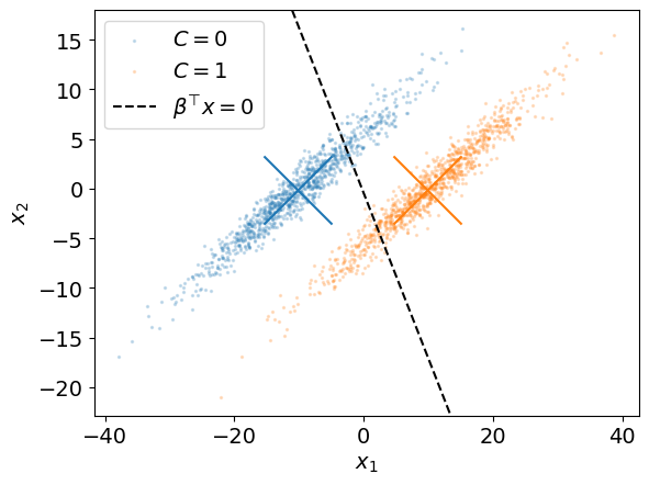
../_images/31fd9965c130cdc224fd9ce4e1adcf724fb19b19e078398b2202b9f905bdc369.png

Once we have determined \(\boldsymbol \beta\), we can project the dataset onto it.

Doing so, the feature space is reduced to a single dimension.

This is illustrated below for our example.

# Project inputs on beta
z1_proj = z1 @ beta
z2_proj = z2 @ beta

fig, ax = plt.subplots(1)
ax.hist(z1_proj, bins, density=density, alpha=alpha_hist,
        label=CLASS_LABELS[0])
ax.hist(z2_proj, bins, density=density, alpha=alpha_hist,
        label=CLASS_LABELS[1])
ax.set_xlabel(r'$\beta^\top x$')
_ = ax.legend()

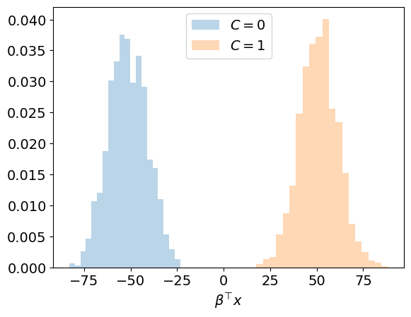
../_images/f2277b48dbf10f989d62550505bc5c65acac8f6344cafdbb4269e099d1ebb598.png

Interpretation:

The inputs associated with the two classes are clearly separated in the one-dimensional space defined by \(\boldsymbol \beta\).

Remark:

Fisher’s linear discriminant, although strictly it is not a discriminant but rather a speciﬁc choice of direction for projection of the data down to one dimension.
However, the projected data can subsequently be used to construct a discriminant, by choosing a threshold for \(\boldsymbol \beta^\top \boldsymbol x\), for instance using standard linear discriminant analysis Classification I: Generative models.

To go further#

Fisher’s linear discriminant can be generalized to any number \(K\) of classes and for \(p\) dimensions provided that \(K \le p\) and that \(q \le K - 1\), with \(q\) the dimension of the reduced space. (Chap. 4 in Bishop 2006).