Overfitting/Underfitting and Bias/Variance

Prerequisites

• Elements of Probability Theory

• Define a supervized-learning problem

• Define and solve an Ordinary Least Squares problem

Learning Outcomes

• Understand when and why a model does or does not generalize well on unseen data

• Understand the difference between the train error and the prediction error.

• Understand overfitting-underfitting and bias-variance tradeoffs

Overfitting and Underfitting

Which fit do you prefer?

Which model performs better on new data?

A harder example:

Varying model complexity

• Data generated by a random process

  • Sample a value of \(X\)

  • Transform with 9th-degree polynomial

  • Add noise to get samples of \(Y\)

Varying model complexity

• Data generated by a random process

• In fact, this process is unknown

• We can only access observations

Varying model complexity

• Data generated by a random process

• In fact, this process is unknown

• We can only access observations

• Fit polynomials of various degrees

Varying model complexity

• Data generated by a random process

• In fact, this process is unknown

• We can only access observations

• Fit polynomials of various degrees

Varying model complexity

• Data generated by a random process

• In fact, this process is unknown

• We can only access observations

• Fit polynomials of various degrees

Varying model complexity

• Data generated by a random process

• In fact, this process is unknown

• We can only access observations

• Fit polynomials of various degrees

Varying model complexity

• Data generated by a random process

• In fact, this process is unknown

• We can only access observations

• Fit polynomials of various degrees

Overfit: model too complex

Model too complex for the data:

• Its best fit would approximate well the process

• However, its flexibility captures noise

Not enough data - Too much noise

Underfit: model too simple

Model too simple for the data:

• Best fit would not approximate well the process

• Yet it captures little noise

Plenty of data - Low noise

Partial Summary

• Models too complex for the data overfit:

  • they explain too well the data that they have seen

  • they do not generalize

• Models too simple for the data underfit:

  • they capture no noise

  • they are limited by their expressivity

Comparing Train and Test Errors

Train vs Test (Prediction) Error

• Error for \(\hat{f}\) from train data \((\mathbf{x}_i, y_i), 1 \le i \le N\):

(35)\[\begin{equation} \overline{\mathrm{err}}_{\hat{f}} = \frac{1}{N} \sum_{i = 1}^N L(y_i, \hat{f}(\mathbf{x}_i)) \end{equation}\]

• Error on the test data (generalization):

(36)\[\begin{equation} \mathrm{Err}_\hat{f} = \mathbb{E}\left[L(Y, \hat{f}(\boldsymbol{X})) | \hat{f}\right] \end{equation}\]

• The EPE is the expectation of \(\mathrm{Err}_\hat{f}\) over all possible train data.

• The train error is easy to estimate but does not tell us much:

  • there is always a model that is sufficiently complex to predict the training data perfectly (e.g. 1-nearest neighbors, Legendre approximating polynomials, deep-enough neural network, etc.)

  • but too complex models overfit

• It is the test error that evaluates how the model performs on new data

• It can be estimated:

  • on some data spared from the training (test data)

  • using more advanced methods such as cross-validation (see Tutorial: Overfitting/Underfitting and Bias/Variance)

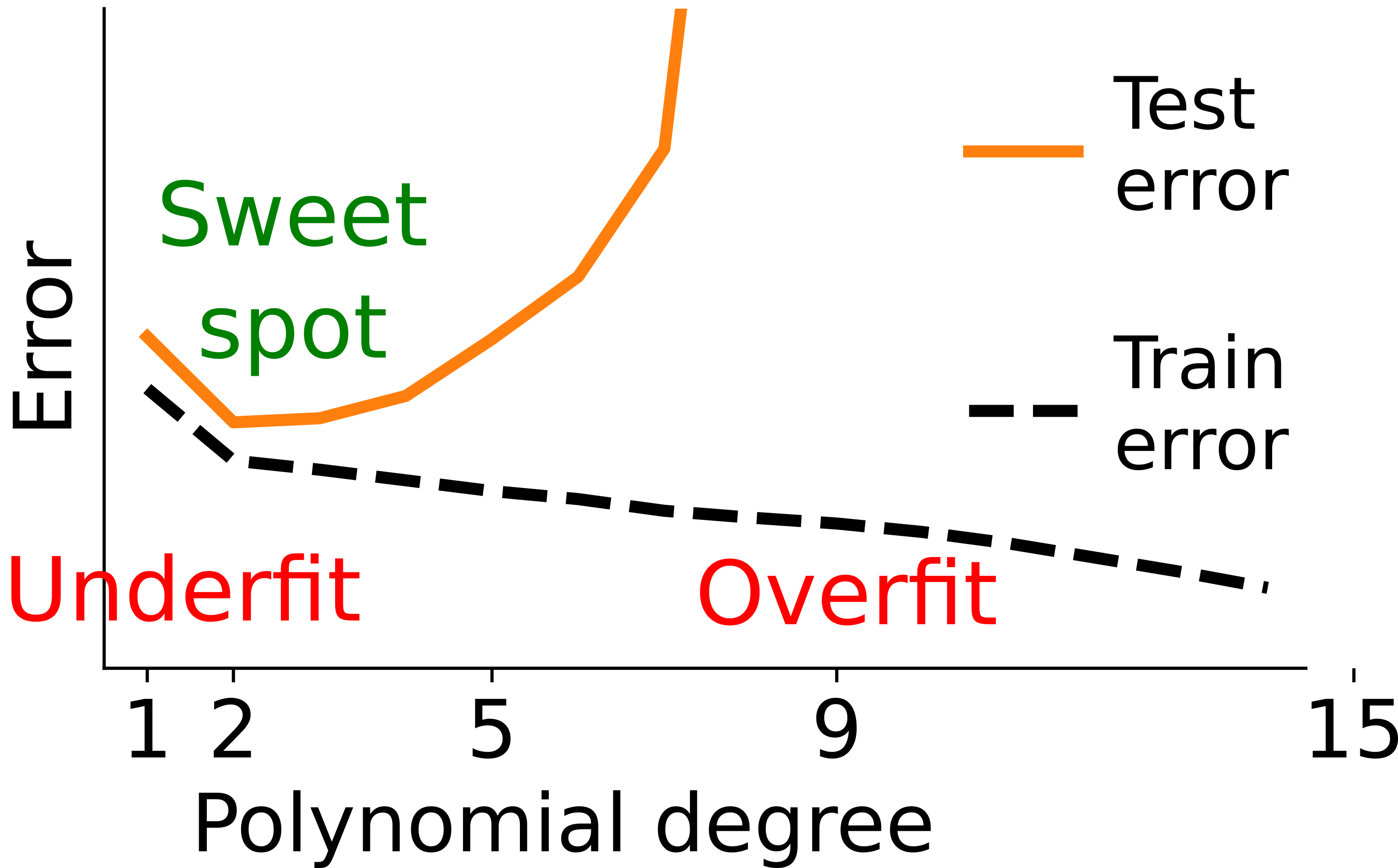
Train vs test error: increasing complexity

Train vs test error: increasing complexity

Train vs test error: increasing complexity

Train vs test error: increasing complexity

Train vs Test Error: Validation Curve

Train vs Test Error: Varying Sample Size

Overfit

Train vs Test Error: Varying Sample Size

Overfit less

Train vs Test Error: Varying Sample Size

Sweet spot?

Train vs Test Error: Learning Curve

Diminishing returns → Try more complex models?

Irreducible Error

Error of best model trained on unlimited data

Here, the data-generating process is a degree-9 polynomial

A higher-degree polynomial will not do better

Predictions limited by noise

Model Families

Crucial to match:

• statistical model

• data-generating process

So far: polynomial for both

Some family names: linear models, decision trees, random forests, kernel machines, multi-layer perceptrons

Different Model Families

• Different inductive (learning) bias

• Different notion of complexity

Different Model Families

Simple variant

Complex variant

Partial Summary

Models overfit:

• number of samples in the training set is too small for model’s complexity

• testing error is much bigger than training error

Models underfit:

• models fail to capture the shape of the training set

• even the training error is large

Different model families = different complexity

Bias versus Variance

Resampling the Training Set

A visual representation of selecting a random sample.
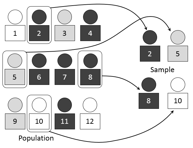
By Dan Kernler - Own work, CC BY-SA 4.0

• A limited amount of training data

• Training set is a small random subset
  of all possible observations

• What is the impact of this choice of training set
  on the learned prediction function?

Practice: Varying Sample Size, Noise Level and Complexity

The following plot represents a 8th-order polynomial to which Gaussian noise is added and to which a polynomial is fitted by OLS.

Question

• Explain changes in the fits depending on the sample size \(N\), noise level \(\sigma\) and model complexity \(m\) in terms of bias (mean error) and variance of the predictions.

from sklearn import linear_model
# Import modules
from pathlib import Path
import numpy as np
import pandas as pd
import holoviews as hv
hv.extension('bokeh')
import hvplot.pandas
import panel as pn

N = 100
M = 7
sc = 0.6
roots = np.linspace(-1 / sc, 1. / sc, M)
xlim = [-1.5, 1.5]
ylim = [-3, 3]
def poly(beta, x):
    m = len(beta)
    monomials = x**np.arange(m)
    return beta @ monomials
def poly_roots(roots, x):
    return np.prod(x - roots) + x


def plot(b, N=100, sigma=0.5, m=1):
    x = np.sort(np.random.randn(N))
    eps = np.random.randn(N)
    fx = np.array([poly_roots(roots, x[i]) for i in range(len(x))])
    ok = (fx > ylim[0]) & (fx < ylim[1])
    x = x[ok]
    fx = fx[ok]
    
    x0 = np.linspace(*xlim, 100)
    fx0 = np.array([poly_roots(roots, x0[i]) for i in range(len(x0))])
    sy_truth = pd.Series(fx0, index=x0)
    sy_truth.name = 'f(x)'
    
    reg = linear_model.LinearRegression(fit_intercept=False)
    X = np.array([x**i for i in range(m + 1)]).T

    eps = eps[ok]
    y = fx + sigma * eps
    sy = pd.Series(y, index=x)
    sy.index.name = 'x'
    sy.name = 'y'
    
    reg.fit(X, y)
    X0 = np.array([x0**i for i in range(m + 1)]).T
    sy_pred = pd.Series(reg.predict(X0), index=x0)
    sy_pred.name = "f'(x)"
    title = "f'(x) = " + '+'.join(
        '{}*x^{}'.format(str(np.round(reg.coef_[i], 1)), i)
        for i in range(len(reg.coef_)))
    
    return sy_truth.hvplot(
        color='k', line_dash='dashed', line_width=3) * sy.hvplot.scatter(
        title=title, xlim=xlim, ylim=ylim, color='k') * sy_pred.hvplot(
        color=hv.Cycle.default_cycles['default_colors'][0], line_width=3)
    
button = pn.widgets.Button(name='Resample', button_type='primary')
pn.interact(plot, b=button, N=np.arange(10, 310, 10),
            sigma=np.arange(0., 1., 0.1), m=np.arange(0, 9))

Overfit: variance

Overfit: variance

Overfit: variance

Overfit: variance

Underfit: bias

Underfit: bias

Underfit: bias

Underfit: bias

Underfit versus Overfit

Underfit

Overfit

Bias-Variance Decomposition of the EPE (Univariate)

We assume that

\[ Y = g(X) + \varepsilon, \]

where \(\mathbb{E}(\varepsilon) = 0\) and \(\mathrm{Var}(\varepsilon) = \sigma_\varepsilon^2\).

The EPE at a new point \(X = x_0\) for a model \(f\) is

\[\mathrm{EPE}(f, x_0) = \mathbb{E}[(Y - \hat{f}(x_0))^2 | X = x_0)],\]

where the expectation is taken with respect to the distribution of the train datasets (i.e. over all fits \(\hat{f}\) of \(f\)) and to the distribution of the output conditioned on \(x_0\).

Question (optional)

• Show that $\( \mathrm{EPE}(f, x_0) = \sigma_\varepsilon^2 + \mathrm{Bias}^2[\hat{f}(x_0)] + \mathrm{Var}[\hat{f}(x_0)], \)$ where

  • \(\mathrm{Bias}^2[\hat{f}(x_0)] = \{\mathbb{E}[\hat{f}(x_0) - g(x_0)]\}^2 = \{\mathbb{E}[\hat{f}(x_0)] - g(x_0)\}^2\),

  • \(\mathrm{Var}[\hat{f}(x_0)] = \mathbb{E}[(\hat{f}(x_0) - \mathbb{E}[\hat{f}(x_0)])^2]\).

Question

• What kind of error does each of these 3 terms represent?

Validation curve.

Learning curve.

Question

• Interpret the validation and learning curves above based on the bias-variance decomposition.

Bias-Variance Decomposition for the OLS

Question (optional)

• Show that, the in-sample error is given by $\( \frac{1}{N}\sum_{i = 1}^N \mathrm{EPE}(f, x_i) = \sigma_\varepsilon^2 + \frac{1}{N} \sum_{i = 1}^N \{\mathbb{E}[\hat{f}(x_i)] - g(x_i)\}^2 + \frac{p}{N} \sigma_\varepsilon^2. \)$

Question

• What kind of error does each of these 3 terms represent?

Partial Summary

High bias == underfitting:

• systematic prediction errors

• the model prefers to ignore some aspects of the data

• mispecified models

High variance == overfitting:

• prediction errors without obvious structure

• small change in the training set, large change in model

• unstable models

To Go Further

• Absence of overfitting issue in Bayesian approach (e.g. Chap. 3 in Bishop 2006).

References

• James, G., Witten, D., Hastie, T., Tibshirani, R., n.d. An Introduction to Statistical Learning, 2st ed. Springer, New York, NY.

• Chap. 2, 3 and 7 in Hastie, T., Tibshirani, R., Friedman, J., 2009. The Elements of Statistical Learning, 2nd ed. Springer, New York.

• Chap. 5 and 7 in Wilks, D.S., 2019. Statistical Methods in the Atmospheric Sciences, 4th ed. Elsevier, Amsterdam.

---

Credit

Contributors include Bruno Deremble and Alexis Tantet. Several slides and images are taken from the very good Scikit-learn course.

---

This work is licensed under a   Creative Commons Attribution-ShareAlike 4.0 International License.