Regularization, Model Selection and Evaluation

Regularization, Model Selection and Evaluation#

Prerequisites

Elements of Probability Theory
Understand the overfitting-underfitting and bias-variance tradeoffs

Learning Outcomes

Estimate the expected prediction error using cross-validation
Use regularization to prevent overfitting
Be aware of underlying statistical assumptions (identity, independence)

Cross-Validation#

Data is often scarce so that living aside test data to estimat the Prediction Error (PE) is a problem
Cross-validation is used to estimate the Expected PE (EPE), while avoiding living aside test data
It uses part of the data to train, part of the data to test, repeating the operation on different subset selections

$K$-Fold Cross Validation#

Slice the train data into $K$ roughly equal-sized parts;
Keep the $K$th part for validation and train on the $K - 1$ other parts;
Compute the prediction error $K$ using the $K$th part;
Repeat the operation for all $K$ parts;
Average the prediction errors to estimate the EPE.

Warning

Cross-validation allows one to estimate expected prediction error rather than the prediction error conditioned on a particular training set (see Chap. 7.12 in Hastie et al. 2009).

Choosing the number $K$ of parts#

$K$ small (e.g. $K = 2$):
biases towards large error (CV training sets size $(K - 1) / K \times N$ much smaller than original training set size $N$);
$K$ large (e.g. $K = N$, leave-one out CV):
unbiased estimate of EPE, but with high variance ($N$ “training sets” are similar to each other);
$K = 5$ or 10:
recommended by Hastie et al. (2009) as a good compromise, but depends on case study.

Adapting Cross-Validation to the Data Structure#

For instance:

By choosing the the number of parts $K$ to adapt to cycles (e.g. avoid splitting years)
By grouping (e.g. if measurements for different people should be kept together)
Shuffling splits (e.g. if the ordering of the data is special)
By taking serial correlations into account in time series.

See https://scikit-learn.org/stable/modules/cross_validation.html#cross-validation-iterators

Regularizing to Avoid Overfitting: Linear Models#

Linear Models Can Overfit#

Linear models are simpler than alternatives
$\rightarrow$ they tend to overfit less than alternatives
They even often underfit when:
- $p$ is small
- the problem is not linearly separable

But linear models can also overfit, when:
- $N$ is small
- Many uninformative features (they depend a lot on other features)

Effect of uninformative features#

Recal that, if we assume that generating model is $Y = \boldsymbol{X}^\top \boldsymbol{\beta} + \epsilon$, where the observations of $\epsilon$ are uncorrelated and with mean zero and constant variance $\sigma^2$, then,

\[\begin{split} \begin{aligned} \mathbb{E}(\hat{\boldsymbol{\beta}} | \mathbf{X}) &= \boldsymbol{\beta}\\ \mathrm{Var}(\hat{\boldsymbol{\beta}} | \mathbf{X}) &= \sigma^2 (\mathbf{X}^\top \mathbf{X})^{-1}. \end{aligned} \end{split}\]

2D example: Assume that, $$ X_1 = c X_0 + (1- c) Z\\ \mathrm{~with~} \mathrm{Var}(X_0) = \mathrm{Var}(Z) = 1 \mathrm{~and~} \mathrm{Cov}(Z, X_0) = 0,\\ \mathrm{Cov}(X_0, Y) = 1 \mathrm{~and~} \mathrm{Cov}(Z, Y) = 0. $$

\[\begin{split} \mathrm{Then,~} \frac{\mathbf{X}^\top \mathbf{X}}{N - 1} \to \begin{pmatrix} 1 & c\\ c & 1 \end{pmatrix} \mathrm{~and~} \frac{\mathbf{X}^\top \mathbf{y}}{N - 1} \to \begin{pmatrix} 1\\ c \end{pmatrix} \mathrm{~when~} N \to \infty. \end{split}\]

\[\begin{split} \mathrm{Thus,~} \left(\frac{\mathbf{X}^\top \mathbf{X}}{N - 1}\right)^{-1} \to \frac{1}{1 - c^2} \begin{pmatrix} 1 & -c\\ -c & 1 \end{pmatrix} \mathrm{~and~} \hat{\boldsymbol{\beta}} \to \begin{pmatrix} 1\\ 0 \end{pmatrix}. \end{split}\]

Example interpretation:

Absolute correlation large $\rightarrow$ large coefficient variance;
Large positive correlation $\rightarrow$ one coefficient large at expense of other.

To go further:

Interpret the role of covariances between inputs in OLS for $M > 2$ using an eigendecomposition of the covariance matrix.

Problem: Many correlated variables $\rightarrow$ high variance.

Origin of the problem: A widely large positive coefficient on one variable can be canceled by a similarly large negative coefficient on its correlated cousin $\rightarrow$ large coefficients.

Idea: weight-decay penalization

Limit the size of the coefficients to reduce the variance of the predictions.

Ridge Regression#

A very common form of regularization for linear regression;
Shrink coefficients by imposing a penalty on their size;
Minimize a penalized RSS:

(37)#\[\begin{equation} \hat{\boldsymbol{\beta}}^\mathrm{ridge} = \underset{\boldsymbol{\beta}}{\mathrm{argmin}} \left\{\sum_{i = 1}^N \left(y_i - \beta_0 - \sum_{j = 1}^p x_{ij} \beta_j \right)^2 + \lambda \sum_{j = 1}^p \beta_j^2 \right\}. \end{equation}\]

$\lambda \ge 0$ controls the amount of shrinkage.

Ridge Regression as a Constrained Optimization#

For any $\lambda$ there exists a $t \ge 0$ such that the ridge regression problem is equivalent to:

(38)#\[\begin{equation} \hat{\boldsymbol{\beta}}^\mathrm{ridge} = \underset{\boldsymbol{\beta}}{\mathrm{argmin}} \sum_{i = 1}^N \left(y_i - \beta_0 - \sum_{j = 1}^p x_{ij} \beta_j \right)^2\\ \mathrm{subject~to~} \sum_{j = 1}^p \beta_j^2 \le t. \end{equation}\]

Warning 1

Contrary to OLS and like in many regularizations, Ridge solutions are not equivarient under scaling:

If different inputs represent different kinds of variables, one normally standardizes the inputs before solving.
If different inputs represent measurements of the same variable in different situations (location, epoch…), it may be interesting to keep the scales.

Warning 2

Penalization of the intercept would make the procedure depend on the origin chosen for $Y$.
After centering the inputs by replacing each $x_{ij}$ by $x_{ij} - \bar{x}_j$, OLS gives $\hat{\beta}_0 = \bar{y}$.
We can thus first solve the ridge for centered inputs and outputs and then add $\hat{\beta}_0 = \bar{y}$ to the predictions.

Question (optional)

Show that the solution to the ridge-penalized RSS is

(39)#\[\begin{equation} \hat{\boldsymbol{\beta}}^\mathrm{ridge} = \left(\mathbf{X}^\top \mathbf{X} + \lambda \mathbf{I}\right)^{-1} \left(\mathbf{X}^\top \mathbf{y}\right), \end{equation}\]

where $\mathbf{I}$ is the $p\times p$ identity matrix.

Question

How does this formula differ from the OLS solution for the coefficients?

When are these solutions unique?

Question (optional)

Show that in the case of orthonormal inputs, the ridge estimates are just a scaled version of the OLS estimates: $\hat{\boldsymbol{\beta}}^\mathrm{ridge} = \hat{\boldsymbol{\beta}} / (1 + \lambda)$.

Question

Use this formula to interpret the effect of the Ridge regularization on the coefficients for orthonormal inputs.

Singular Value Decomposition Interpretation (optional)#

Let the SVD of $\mathbf{X}$ be $\mathbf{X} = \mathbf{U} \mathbf{D} \mathbf{V}^\top$ with:

$\mathbf{U}$ an $N \times p$ orthogonal matrix with columns spanning the column space of $\mathbf{X}$;
$\mathbf{V}$ a $p \times p$ orthogonal matrix with columns spanning the row space of $\mathbf{X}$;
$\mathbf{D}$ a $p \times p$ diagonal matrix with diagonal entries $d_1 \ge d_2 \ge \cdots d_p \ge 0$ called the singular values of $\mathbf{X}$.

Question (optional)

Show that the OLS estimates are such that $\mathbf{X} \hat{\boldsymbol{\beta}} = \mathbf{U} \mathbf{U}^\top \mathbf{y}$.

Show that the ridge estimates are such that $\mathbf{X} \hat{\boldsymbol{\beta}}^\mathrm{ridge} = \sum_{j = 1}^p \mathbf{u}_j \frac{d_j^2}{d_j^2 + \lambda} \mathbf{u}_j^\top \mathbf{y}$.

Question

Interpret how the ridge shrinks the coordinates of $\mathbf{y}$ with respect to the orthonormal basis $\mathbf{U}$.

What is the role of $\mathrm{df}(\lambda) := \mathrm{tr}\left[\mathbf{X}(\mathbf{X}^\top \mathbf{X} + \lambda \mathbf{I})^{-1} \mathbf{X}^\top\right] = \sum_{j = 1}^p \frac{d_j^2}{d_j^2 + \lambda}$.

Regularization on a Simple Example#

Small training set
Fit a linear model without regularization

Regularization on a Simple Example#

Small training set
Fit a linear model without regularization
Training points sampled at random
Can overfit if the data is noisy!

Regularization on a Simple Example: Random Training Sets#

Bias-Variance Tradeoff in Ridge Regression#

Linear regression (OLS)
High variance, no bias

Ridge regression
Low variance, but biased!

Bias-Variance Tradeoff in Ridge Regression#


Too much variance	Best tradeoff	Too much bias

Partial Summary#

Can overfit when:
- $N$ is too small and $p$ is large
- In particular with non-informative features
Regularization for regression:
- From linear regression to ridge regression $\rightarrow$ less overfit
- large regularization parameter $\rightarrow$ strong regularization $\rightarrow$ smaller coefficients

Tuning Hyperparameters (model selection)#

Some hyperparameters need to be estimated in addition to coefficients (regularization parameter, nonlinear coefficients in linear models, etc.)
Validation data or Cross-Validation (CV) may be used to select the best hyperparameters by minimizing the estimated validation error (grid search, random search, etc.)

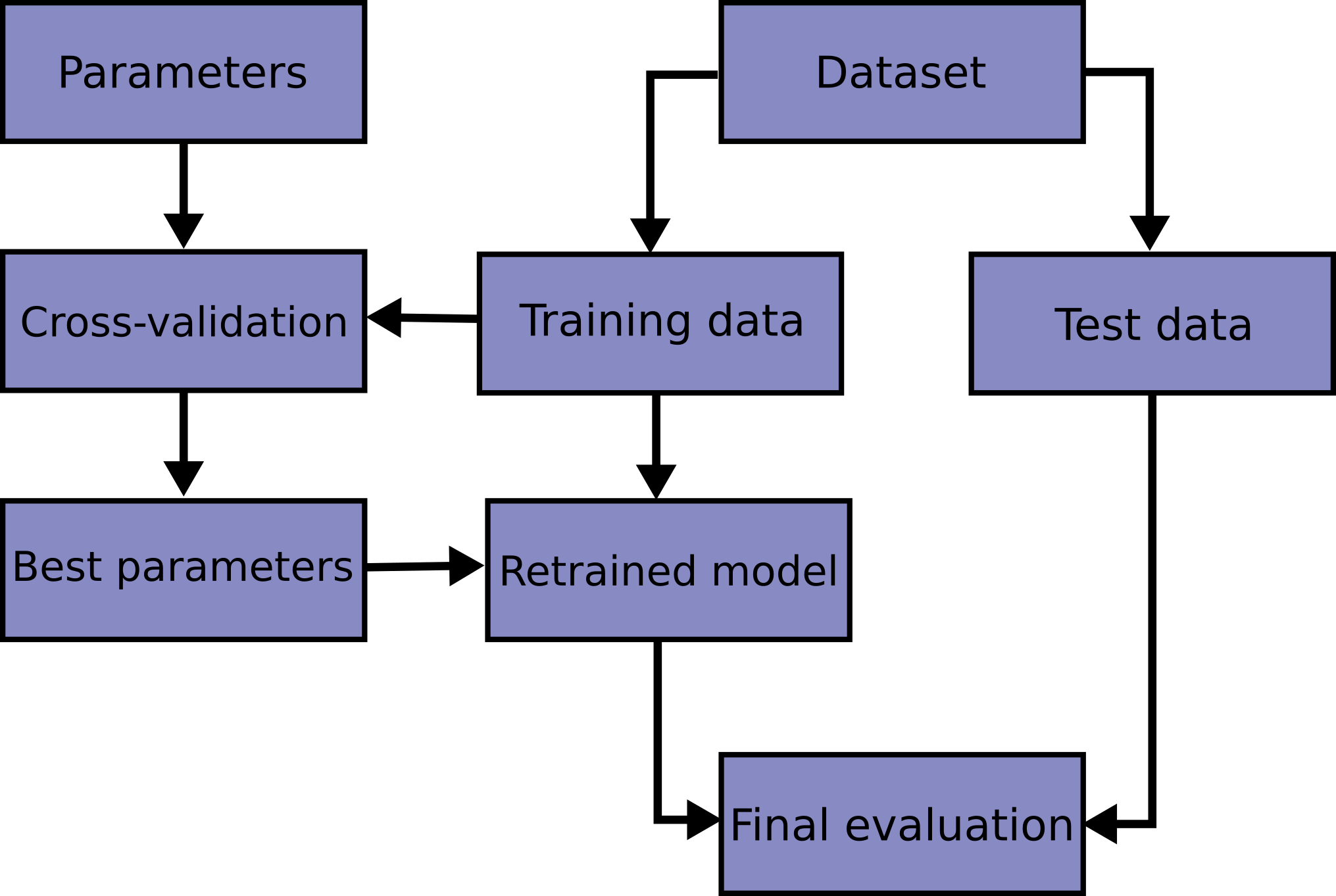
Testing after validation#

The best validation error is for hyperparameters that were trained using the validation data: it is not the EPE for this choice of hyperparameters!

$\rightarrow$ Distinguish between train, validation and test data

Training and validation can be combined using CV but test data should be kept to evaluate the PE conditionned on the CV set for the final choice of coefficients and hyperparameters.

To maximize the use of the data and estimate the EPE, nested CV can be used.

Law of Large Numbers?#

Estimates attempt to minimize a function of the training error $\overline{\mathrm{err}}$.

For estimates to converge with the sample size, so should $\overline{\mathrm{err}}$.

$\rightarrow$ We need some Law of Large Numbers to be applicable.

Basic assumptions: independent and identically distributed.

What could go wrong?#

In the natural and engineering sciences many problems depend on time.

So far, we have assumed that the joint distribution $f_{\boldsymbol{X}, Y}$ is independent of time.

In particular, we have assumed that the joint process is statistically stationary.

Variations in time can rarely be considered purely random:

$\rightarrow$ some dependence persist between realizations

Yet, we are fine if we can show that:

there is a stationary distribution
realizations sufficiently distant in time no longer correlate

However, distributions may change with cycles and trends.

Violation of Statistical Stationarity#

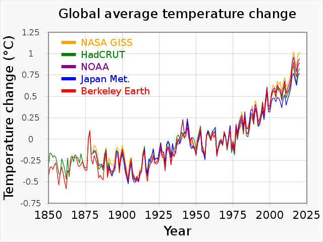
../_images/640px-20200324_Global_average_temperature_-_NASA-GISS_HadCrut_NOAA_Japan_BerkeleyE.svg.png

By RCraig09 - Own work, CC BY-SA 4.0

Surface air temperature variability can be decomposed into:

$-$ (pseudo-)periodic cycles (diurnal, annual, Milankovitch)

$-$ a continuous spectrum of frequencies due to chaotic dynamics

$-$ an increasing trend due to global warming

$-$ other non-equilibrium variations (effect of volcanoes, solar activity, …)

Partial Summary#

In statistics, we always make assumptions about the probability distribution of the data (stationarity, independence, parametric form, etc.)
The quality of statistics (predictions, error estimates, etc.) depends on the validity of these assumptions
Even the best validation could be wrong about predictions if the new data does not satisfy these assumptions!

To go further#

Linear model inspection in Scikit-learn course;
Introduction of the evaluation metrics in Scikit-learn course;
Generalized CV approximation of leave-one out CV (Chap. 7.10 in Hastie et al. 2009);
The bootstrap as a way of assessing the accuracy of a parameter estimate or a prediction (shuffled version of cross-validation, Chap. 7.11 and 8 in Hastie et al. 2009).
Avoiding validation thanks to Bayesian approach.