Tutorial: Ensemble Methods for Wind Capacity Factor Prediction#
![]()
Tutorial to the class Ensemble Methods based on the same case study as in Tutorial: Regularization, Model Selection and Evaluation and Tutorial: Introduction to Unsupervised Learning with a Focus on PCA.
Use ensemble methods to best predict the France-average wind capacity factor from a large number of input variables;
Control the complexity parameter(s) of each ensemble method to avoid overfitting;
Compare the skills of different methods.
Scientific objective#
To predict the France average wind capacity factor from the geopotential height at 500hPa over the Euro-Atlantic sector.
Dataset presentation#
Input:
Geopotential height at 500hPa
Domain: North Atlantic
Spatial resolution: \(0.5° \times 0.625°\)
Time resolution: monthly
Period: 1980-2021
Units: m
Source: MERRA-2 reanalysis
Target:
Onshore wind capacity factors
Domain: Metropolitan France
Spatial resolution: regional mean
Time resolution: daily
Period: 2014-2021
Units:
Source: RTE
Getting ready#
Reading the wind capacity factor and geopotential height data#
We follow the same procedure as in # Tutorial: Regularization, Model Selection and Evaluation.
# Path manipulation module
from pathlib import Path
# Numerical analysis module
import numpy as np
# Formatted numerical analysis module
import pandas as pd
# Structured dataset analysis module
import xarray as xr
# Plot module
import matplotlib.pyplot as plt
# Default colors
RC_COLORS = plt.rcParams['axes.prop_cycle'].by_key()['color']
# Matplotlib configuration
plt.rc('font', size=14)

# Set data directory
data_dir = Path('data')

# Set keyword arguments for pd.read_csv
kwargs_read_csv = dict(index_col=0, parse_dates=True)

# Define electricity demand filepath and label
windcf_filename = 'reseaux_energies_capacityfactor_wind-onshore.csv'
windcf_filepath = Path(data_dir, windcf_filename)
windcf_label = 'Wind capacity factor'

# Read windcf data with pandas
df_windcf_daily = pd.read_csv(windcf_filepath, **kwargs_read_csv)

# Select domain
# REGION_NAME = 'Bretagne'
REGION_NAME = 'National'
if REGION_NAME == 'National':
    df_windcf_daily_reg = df_windcf_daily.mean('columns')
    df_windcf_daily_reg.name = REGION_NAME
else:
    df_windcf_daily_reg = df_windcf_daily[REGION_NAME]

# Resample wind capacity factor from daily to monthly means
df_windcf_reg = df_windcf_daily_reg.resample('MS').mean()

# Define temperature filepath and label
START_DATE = '19800101'
END_DATE = '20220101'
z500_filename = 'merra2_analyze_height_500_month_{}-{}.nc'.format(START_DATE, END_DATE)
z500_filepath = Path(data_dir, z500_filename)
z500_label = 'Geopotential height (m)'

# Read geopotential height dataset with xarray
ds = xr.load_dataset(z500_filepath)

# Select geopotential height variable
z500_name = 'height_500'
da_z500_hr = ds[z500_name]

# Downsample geopotential height
N_GRID_AVG = 8
da_z500 = da_z500_hr.coarsen(lat=N_GRID_AVG, boundary='trim').mean().coarsen(
    lon=N_GRID_AVG, boundary='trim').mean()

# Remove seasonal cycle from wind capacity factor
da_windcf_reg = df_windcf_reg.to_xarray()
gp_windcf_cycle = da_windcf_reg.groupby('time.month')
da_windcf_anom = gp_windcf_cycle - gp_windcf_cycle.mean('time')
df_windcf_anom = da_windcf_anom.drop('month').to_dataframe()[REGION_NAME]

# Remove seasonal cycle from geopotential height or not
gp_z500_cycle = da_z500.groupby('time.month')
da_z500_anom = gp_z500_cycle - gp_z500_cycle.mean('time')

# Convert to bandas with grid points as columns
df_z500_anom = da_z500_anom.stack(latlon=('lat', 'lon')).to_dataframe()[
    z500_name].unstack(0).transpose()

# Select common index
idx = df_z500_anom.index.intersection(df_windcf_anom.index)
df_z500_anom = df_z500_anom.loc[idx]
df_windcf_anom = df_windcf_anom.loc[idx]

# Number of years in dataset
time = df_windcf_anom.index
n_years = time.year.max() - time.year.min() + 1
Ensemble methods#
Regressions evaluation function#
We also define a function to evaluate any of our regressions.
FIRST_TEST_YEAR controls the number of years at the end of the time series to keep as test data.
from sklearn import model_selection
# Default number of test days
FIRST_TEST_YEAR = 2020
POLY_DEGREE = 1
# Get input matrix and output vector for whole time series
X = df_z500_anom.values
y = df_windcf_anom.values
def evaluate_regressor(
reg, reg_kwargs, param_name, param_range, first_test_year=FIRST_TEST_YEAR,
n_splits=None, cv_iterator=model_selection.KFold,
plot_validation=True):
if n_splits is None:
n_splits = len(np.unique(time[time.year < first_test_year].year))
# Get test data keeping last years
index_test = time.year >= first_test_year
X_test = X[index_test]
y_test = y[index_test]
# Select train data from first years and first days in month
index_cv = time.year < first_test_year
X_cv = X[index_cv]
y_cv = y[index_cv]
if plot_validation:
# Set cross-validation iterator
cv = cv_iterator(n_splits=n_splits)
groups = time[index_cv].year
# Get train and validation scores from cross-validation
train_scores, validation_scores = model_selection.validation_curve(
reg, X_cv, y_cv, param_name=param_name,
param_range=param_range, cv=cv, groups=groups)
# Get train curve
train_scores_mean = train_scores.mean(1)
train_scores_max = train_scores.max(1)
train_scores_min = train_scores.min(1)
# Get validation curve
validation_scores_mean = validation_scores.mean(1)
validation_scores_max = validation_scores.max(1)
validation_scores_min = validation_scores.min(1)
# Get best value of the regularization parameter
i_best = np.argmax(validation_scores_mean)
param_best = param_range[i_best]
score_best = validation_scores_mean[i_best]
# Plot validation curve
lw = 2
plt.figure()
plt.semilogx(param_range, train_scores_mean, label="Training score",
color="darkorange", lw=lw)
plt.fill_between(param_range, train_scores_min, train_scores_max,
alpha=0.2, color="darkorange", lw=lw)
plt.semilogx(param_range, validation_scores_mean,
label="Cross-validation score", color="navy", lw=lw)
plt.fill_between(
param_range, validation_scores_min, validation_scores_max,
alpha=0.2, color="navy", lw=lw)
plt.xlabel(param_name)
plt.ylabel(r'Validation $R^2$')
plt.xlim(param_range[[0, -1]])
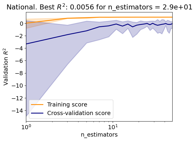
plt.title(REGION_NAME + r'. Best $R^2$: {:.2} for {} = {:.1e}'.format(
score_best, param_name, param_best))
# plt.ylim(0.0, 1.1)
plt.legend(loc="best")
# Set best parameter
reg.set_params(**{param_name: param_best})
else:
param_best = reg.get_params(param_name)
# Compute prediction error conditioned on first 5 years of data
reg.fit(X_cv, y_cv)
test_score = reg.score(X_test, y_test)
print('\nTest R2: {:.2f}'.format(test_score))
# Predict for work days and off days
y_pred = reg.predict(X_test)
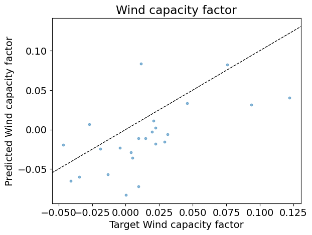
# Scatter plot of prediction against target
fig, ax = plt.subplots()
ax.scatter(y_test, y_pred, s=10, alpha=0.5)
xlim = ax.get_xlim()
ax.plot(xlim, xlim, '--k', linewidth=1)
ax.set_xlabel('Target ' + windcf_label)
ax.set_ylabel('Predicted ' + windcf_label)
ax.set_xlim(xlim)
ax.set_title('Wind capacity factor')
return {param_name: param_best}
Question
If 2021 is given as the first test years, how many training years and test years will be available for this dataset?
Identify the lines where:
The validation and train scores are computed;
The test score is computed;
The target is predicted from the test input features.
Answer:
Individual models#
First, make sure that only the heating and cooling temperatures are selected as features, that the monthly factorization is activated and that no polynomial transformation is performed.
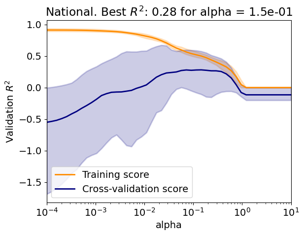
Lasso regression#
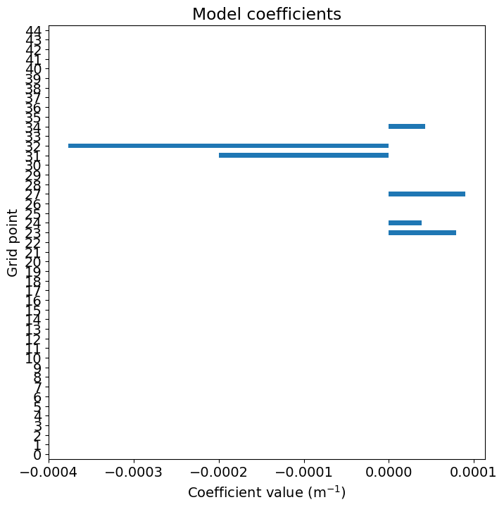
The following code:
Creates a Lasso regressor with positive coefficients;
Evaluate the regressor over a range of regularization parameter values;
Represent the importance of the coefficients.
The evaluation function:
Plots the training and validation curves with the lines representing the mean score and the shading the minimum and maximum scores;
Plots test predictions against the test inputs over the train data;
Plots the test predictions against the test targets.
Question
Is there an overfit/underfit tradeoff?
Explain the difference between the training curve and the validation curve?
Explain the evolution the variability of the validation curve.
Is the test score in agreement with the best validation score?
How does the the importance of the coefficients vary with climate variable and the month?
from sklearn import linear_model

# Define array of complexity coordinate, regressor and options
# for Lasso regression
param_name, param_range = 'alpha', np.logspace(-4, 1, 50)
reg_kwargs_lasso = dict(max_iter=10000)
reg_lasso = linear_model.Lasso(
    **{param_name: param_range[0]}, **reg_kwargs_lasso)

# Evaluate regressor
param_best_lasso = evaluate_regressor(
    reg_lasso, reg_kwargs_lasso, param_name, param_range)
df_coef = pd.Series(reg_lasso.coef_)
plt.figure()
df_coef.plot(kind='barh', figsize=(8, 8))
plt.xlabel(r'Coefficient value (m$^{-1}$)')
plt.ylabel('Grid point')
_ = plt.title('Model coefficients')
Test R2: 0.31

Answer:
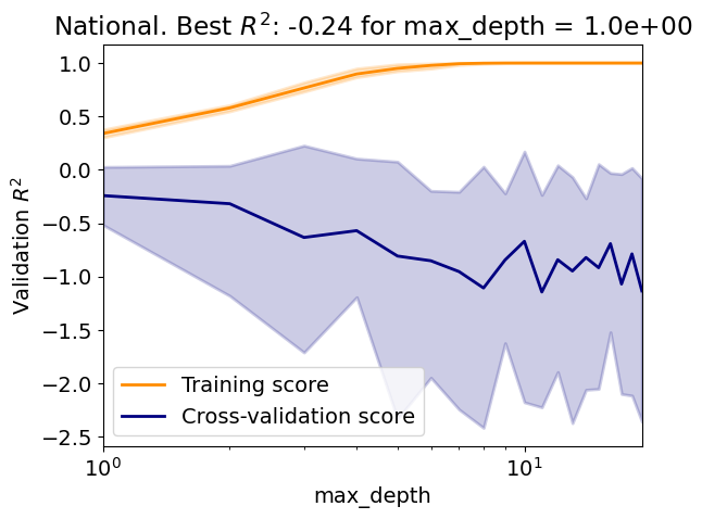
Decision-tree regression#
The following code:
Creates a decision-tree regressor;
Evaluate the regressor over a range of maximum tree depth;
Question
Is there an overfit/underfit tradeoff?
How does the tree perform compared to the Lasso?
from sklearn import tree

# Define array of complexity coordinate, regressor and options
# for decision-tree regression
param_name, param_range = 'max_depth', np.arange(1, 20, 1)
reg_kwargs_dt = dict()
reg_dt = tree.DecisionTreeRegressor(
    **{param_name: param_range[0]}, **reg_kwargs_dt)

# Evaluate regressor
param_best_dt = evaluate_regressor(
    reg_dt, reg_kwargs_dt, param_name, param_range)
Test R2: -0.01

Answer:
Ensemble models#
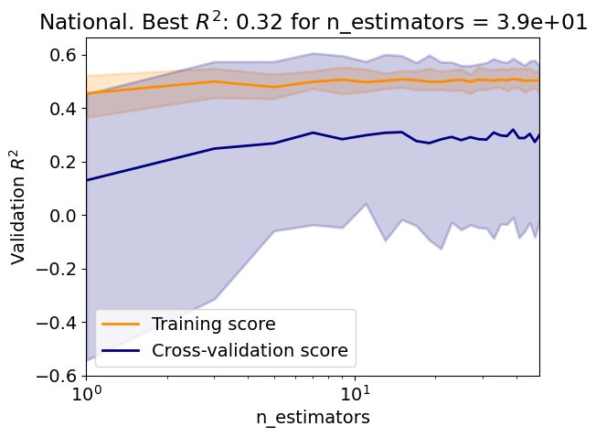
Bagging regressor#
The following code:
Creates a bagging regressor with a decision tree as the base estimator;
Evaluate the regressor over a range of number of estimators;
Question
Use the Scikit-learn documentation to give the parameters defining this bagging regressor with a decision tree as the base estimator.
Question
Is there an overfit/underfit tradeoff?
In this case, how to choose the number of estimators?
Same question without using validation curves.
How does the bagging perform compared to the individual regressors?
Same question but with the Lasso as base estimator.
from sklearn import ensemble

# Define array of complexity coordinate, regressor and options
# for Bagging regression
param_name, param_range = 'n_estimators', np.arange(1, 50, 2)
# estimator = None
estimator = linear_model.Lasso(alpha=0.15)
reg_kwargs_br = dict(estimator=estimator)
reg_br = ensemble.BaggingRegressor(
    **{param_name: param_range[0]}, **reg_kwargs_br)

# Evaluate regressor
param_best_br = evaluate_regressor(
    reg_br, reg_kwargs_br, param_name, param_range)
Test R2: 0.32
Answer:
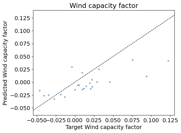
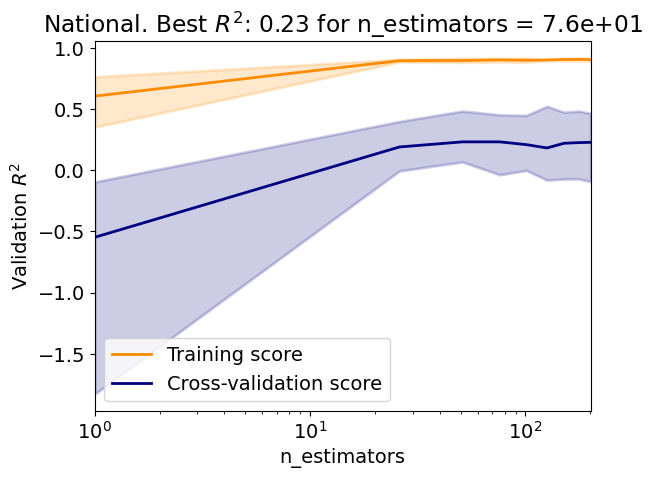
Random-forest regressor#
The following code:
Creates a random-forest regressor;
Evaluate the regressor over a range of number of estimators;
Question
Use the Scikit-learn documentation to give the parameters defining this random-forest regressor.
Question
How does the random forest perform compared to the bagging regressor?
Compare the varibility of the validation score of the random forest to that of the bagging regressor.
# Define array of complexity coordinate, regressor and options
# for random-forest regression
param_name, param_range = 'n_estimators', np.arange(1, 202, 25)
reg_kwargs_rf = dict()
reg_rf = ensemble.RandomForestRegressor(
    **{param_name: param_range[0]}, **reg_kwargs_rf)

# Evaluate regressor
param_best_rf = evaluate_regressor(
    reg_rf, reg_kwargs_rf, param_name, param_range)
Test R2: 0.06

Answer:
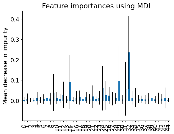
The following plot represents the mean and standard deviation of the importance given to the features by the trees in the random forest (see Feature importance with a forest of trees in Scikit-learn User guide).
Question
How does the the importance of the features vary with climate variable and the month?
Compare the importance of the random-forest features with that of the Lasso.
# Plot importance
importances = reg_rf.feature_importances_
std = np.std([tree.feature_importances_ for tree in reg_rf.estimators_], axis=0)
forest_importances = pd.Series(importances)

fig, ax = plt.subplots()
forest_importances.plot.bar(yerr=std, ax=ax)
ax.set_title("Feature importances using MDI")
_ = ax.set_ylabel("Mean decrease in impurity")
Answer:
Voting regressor#
The following code creates a voting regressor with the Lasso, the decision tree and the random forest as base estimators and tests it.
Question
Use the Scikit-learn documentation to give the parameters defining this voting regressor.
Question
How does the voting regressor perform compared to the base estimators?
# Define array of complexity coordinate, regressor and options
# for voting regression
param_name, param_range = 'estimators', [
    [('Lasso', reg_lasso), ('DecisionTree', reg_dt), ('RandomForest', reg_rf)]
]
reg_kwargs_vr = dict()
reg_vr = ensemble.VotingRegressor(
    **{param_name: param_range[0]}, **reg_kwargs_vr)

# Evaluate regressor
param_best_vr = evaluate_regressor(
    reg_vr, reg_kwargs_vr, param_name, param_range,
    plot_validation=False)
Test R2: 0.23
Answer:
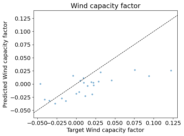
Stacking regressor#
The following code creates a stacking regressor with the Lasso, the decision tree and the random forest as base estimators and tests it.
The final regressor is a OLS with positive coefficients.
The weights given to the base estimators by the stacking are also given.
Question
Use the Scikit-learn documentation to give the parameters defining this stacking regressor.
Question
How does the stacking regressor perform compared to the voting regressor? Why?
# Define array of complexity coordinate, regressor and options
# for voting regression
param_name, param_range = 'estimators', [
    [('Lasso', reg_lasso), ('DecisionTree', reg_dt), ('RandomForest', reg_rf)]
]
reg_kwargs_sr = dict(final_estimator=linear_model.LinearRegression(
    positive=True))
reg_sr = ensemble.StackingRegressor(
    **{param_name: param_range[0]}, **reg_kwargs_sr)

# Evaluate regressor
param_best_sr = evaluate_regressor(
    reg_sr, reg_kwargs_sr, param_name, param_range, plot_validation=False)
weights = reg_sr.final_estimator_.coef_
index = [r[0] for r in param_range[0]]
df_weights = pd.Series(weights, index=index)
print('Weights:')
print(df_weights)
Test R2: 0.23
Weights:
Lasso           0.877058
DecisionTree    0.000000
RandomForest    0.076595
dtype: float64

Answer:
AdaBoost regressor#
The following code:
Creates an AdaBoost regressor;
Evaluate the regressor over a range of number of estimators;
Question
Use the Scikit-learn documentation to give the parameters defining this AdaBoost regressor.
Question
How does the AdaBoost compared to the other regressors?
# Define array of complexity coordinate, regressor and options
# for AdaBoost regression
param_name, param_range = 'n_estimators', np.arange(1, 50, 2)
estimator = linear_model.LinearRegression(fit_intercept=True)
reg_kwargs_abr = dict(estimator=estimator)
reg_abr = ensemble.AdaBoostRegressor(
    **{param_name: param_range[0]}, **reg_kwargs_abr)

# Evaluate regressor
param_best_abr = evaluate_regressor(
    reg_abr, reg_kwargs_abr, param_name, param_range)
Test R2: -0.21
Question (Optional)
Reevaluate your results for a different scoring metric.
Answer:
Credit#
Contributors include Bruno Deremble and Alexis Tantet. Several slides and images are taken from the very good Scikit-learn course.
