Appendix: Elements of Probability Theory

Appendix: Elements of Probability Theory#

Probability Measures#

Sample Space
The set of all possible outcomes of an experiment is called the sample space and is denoted by \(\Omega\).

\(Events\) are defined as subsets of the sample space.

\(\sigma\)-algebra
A collection \(\mathcal{F}\) of sets in \(\Omega\) is called a \(\sigma\)-algebra on \(\Omega\) if

\(\emptyset \in \mathcal{F}\);
if \(A \in \mathcal{F}\), then \(A^c \in \mathcal{F}\);
if \(A_1, A_2, \ldots \in \mathcal{F}\), then \(\cup_{i = 1}^\infty A_i \in \mathcal{F}\).

Generated \(\sigma\)-algebra
The intersection of all the \(\sigma\)-algebras containing \(\mathcal{F}\), denoted \(\sigma(\mathcal{F})\), is a \(\sigma\)-algebra that we call the \(\sigma\)-algebra generated by \(\mathcal{F}\).

Borel \(\sigma\)-algebra
Let \(\Omega = \mathbb{R}^p\). The \(\sigma\)-algebra generated by the open subsets of \(\mathbb{R}^p\) is called the Borel \(\sigma\)-algebra of \(\mathbb{R}^p\) and is denoted by \(\mathcal{B}(\mathbb{R}^p)\).

The \(\sigma\)-algebra of a sample space contains all possible outcomes of the experiment that we want to study.

Intuitively, the \(\sigma\)-algebra contains all the useful information that is available about the random experiment that we are performing.

Probability Measure
A probability measure \(\mathbb{P}\) on the measurable space \((\Omega, \mathcal{F})\) is a function \(\mathbb{P}: \mathcal{F} \to [0, 1]\) satisfying

\(\mathbb{P}(\emptyset) = 0\), \(\mathbb{P}(\Omega) = 1\);
For \(A_1, A_2, \ldots\) with \(A_i \cap A_j = \emptyset\), \(i \ne j\), then

(170)#\[\begin{equation} \mathbb{P}(\cup_{i = 1}^\infty A_i) = \sum_{i = 1}^\infty \mathbb{P}(A_i) \end{equation}\]

Probability Space
The triple \((\Omega, \mathcal{F}, \mathbb{P})\) comprising a set \(\Omega\), a \(\sigma\)-algebra \(\mathcal{F}\) of subsets of \(\Omega\) and a probability measure \(\mathbb{P}\) on \((\Omega, \mathcal{F})\) is called a probability space.

Independent Sets
The sets \(A\) and \(B\) are \(independent\) if

(171)#\[\begin{equation} \mathbb{P}(A \cap B) = \mathbb{P}(A) \mathbb{P}(B). \end{equation}\]

Random Variables#

Measurable Space
A sample space \(\Omega\) equipped with a \(\sigma\)-algebra of subsets \(\mathcal{F}\) is called a measurable space.

../_images/Random_Variable_as_a_Function-en.svg

This graph shows how random variable is a function from all possible outcomes to real values.
It also shows how random variable is used for defining probability mass functions.
By Niyumard - Own work, CC BY-SA 4.0

Random Variable and Random Vector
Let \((\Omega, \mathcal{F})\) and \((\mathbb{R}^p, \mathcal{B}(\mathbb{R}^p))\) be two measurable spaces. Is called a measurable function or random variable (\(p = 1\)) or random vector (\(p > 1\)) a function \(\boldsymbol{X}: \Omega \to \mathbb{R}^p\) such that the event

\(\{\omega \in \Omega: X_1(\omega) \le x_1, \ldots, X_p(\omega) \le x_p\}\) \(=: \{\omega \in \Omega: \boldsymbol{X}(\omega) \le \boldsymbol{x}\}\) \(=: \{\boldsymbol{X} \le \boldsymbol{x}\}\)

belongs to \(\mathcal{F}\) for any \(\boldsymbol{x} \in \mathbb{R}^p\).

In other words, the preimage of any Borel set under \(\boldsymbol{X}\) is an event.

Cumulative distribution function for the normal distribution.
By Inductiveload - self-made, Mathematica, Inkscape, Public Domain

Distribution Function of a Random Variable
Every random variable from a probability space \((\Omega, \mathcal{F}, \mu)\) to \((\mathbb{R}, \mathcal{B}(\mathbb{R}))\) induces a probability measure \(\mathbb{P}\) on \(\mathbb{R}\) that we identify with the probability distribution function \(F_X: \mathbb{R} \to [0, 1]\) defined as

\(F_X(x) = \mu(\omega \in \Omega: X(\omega) \le x)\) \(=: \mathbb{P}(X \le x), x \in \mathcal{B}(\mathbb{R})\).

In this case, \((\mathbb{R}, \mathcal{B}(\mathbb{R}), F_X)\) becomes a probability space.

If \(X\) is not a measurable function, there exists an \(x\) in \(\mathbb{R}\) such that \(\{\omega \in \Omega: X \le x\}\) is not an event. Then, \(\mathbb{P}(X \le x) = \mu(\omega \in \Omega: X \le x)\) is not defined and we cannot define the distribution of \(X\).

This shows that it is the measurability of a random variable that makes it so special.

../_images/Multivariate_normal_sample.svg

Many sample observations (black) drawn from a joint probability distribution.
The marginal densities are shown as well.
By IkamusumeFan - Own work, CC BY-SA 3.0

Joint Distribution Function
Let \(X\) and \(Y\) be two random variables. We can then define their joint distribution function as

(172)#\[\begin{equation} F_{X, Y}(x, y) = \mathbb{P}(X \le x, Y \le y) \end{equation}\]

We can view them as a random vector, i.e. a random variable from \(\Omega\) to \(\mathbb{R}^2\).

Independent Random Variables
Two random variables \(X\) and \(Y\) on \(\mathbb{R}\) are independent if the events \(\{\omega \in \Omega: X(\omega) \le x\}\) and \(\{\omega \in \Omega: Y(\omega) \le y\}\) are independent for all \(x, y \in \mathbb{R}\).

If \(X\) and \(Y\) are independent then \(F_{X, Y}(x, y) = F_X(x)F_Y(y)\).

Distribution Function of a Random Vector
Every random variable from a probability space \((\Omega, \mathcal{F}, \mu)\) to \((\mathbb{R}^p, \mathcal{B}(\mathbb{R}^p))\) induces a probability measure \(\mathbb{P}\) on \(\mathbb{R}^p\) that we identify with the distribution function \(F_\boldsymbol{X}: \mathbb{R}^p \to [0, 1]\) defined as

(173)#\[\begin{equation} F_\boldsymbol{X}(\boldsymbol{x}) = \mathbb{P}(\boldsymbol{X} \le \boldsymbol{x}) := \mu(\omega \in \Omega: \boldsymbol{X}(\omega) \le \boldsymbol{x}) \ \ \ \ \boldsymbol{x} \in \mathcal{B}(\mathbb{R}^p). \end{equation}\]

Expectation of Random Variables
Let \(X\) be a random variable from \((\Omega, \mathcal{F}, \mu)\) to \((\mathbb{R}^p, \mathcal{B}(\mathbb{R}^p))\). We define the expectation of \(\boldsymbol{X}\) by

(174)#\[\begin{equation} \mathbb{E}(\boldsymbol{X}) = \int_{\mathbb{R}^p} \boldsymbol{x} dF_\boldsymbol{X}(\boldsymbol{x}). \end{equation}\]

More generally, let \(f: \mathbb{R}^p \to \mathbb{R}\) be measurable. Then

(175)#\[\begin{equation} \mathbb{E}(f(\boldsymbol{X})) = \int_{\mathbb{R}^p} f(\boldsymbol{x}) dF_\boldsymbol{X}(\boldsymbol{x}). \end{equation}\]

\(dF_\boldsymbol{X}(\boldsymbol{x}) = \mathbb{P}(d\boldsymbol{x}) = \mathbb{P}(dx_1, \ldots, dx_p)\) and \(\int\) denotes the Lebesgue integral.

When a function is continuous, its Lebesgue integral can be replaced by its Riemann-Stieltjes integral.

\(L^p\) spaces
By \(L^p(\Omega, \mathcal{F}, \mu)\) we mean the Banach space of measurable functions on \(\Omega\) with norm

(176)#\[\begin{equation} \|X\|_{L^p} = \left(E(|X|^p)\right)^{1/p}. \end{equation}\]

In particular, we say that \(X\) is integrable if \(\|X\|_{L^1} < \infty\) and that \(X\) has finite variance if \(\|X\|_{L^2} < \infty\).

Variance, Covariance and Correlation of Two Random Variables#

Variance of a Random Variable
Provided that it exists, we define the variance of a random variable \(X\) as

(177)#\[\begin{equation} \mathrm{Var}(X) := \mathbb{E}\left[(X - \mathbb{E}(X))^2\right] = \mathbb{E}(X^2) - \mathbb{E}(X)^2. \end{equation}\]

../_images/1024px-Correlation_examples2.svg.png

Several sets of (X, Y) points, with the corresponding Pearson
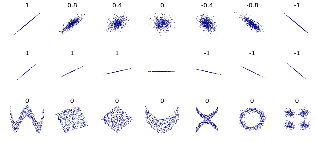
correlation coefficient. The correlation reflects the noisiness and
direction of a linear relationship (top row), but not the slope of that
relationship (middle), nor many aspects of nonlinear relationships (bottom).
N.B.: the figure in the center as a slope of 0 but in that case the
correlation coefficient is undefined because the variance of Y is zero.
DenisBoigelot, original uploader was Imagecreator

Covariance, Variance and Correlation of Two Random Variables
Provided that it exists, we define the covariance of two random variables \(X\) and \(Y\) as

\(\mathrm{Cov}(X, Y) := \mathbb{E}\left[(X - \mathbb{E}(X)) (Y - \mathbb{E}(Y))\right]\) \(= \mathbb{E}(X Y) - \mathbb{E}(X) \mathbb{E}(Y).\)

The correlation of \(X\) and \(Y\) is

\(\mathrm{Corr}(X, Y) := \frac{\mathrm{Cov}(X, Y)}{\sqrt{\mathrm{Var}(X)} \sqrt{\mathrm{Var}(Y)}}.\)

Conditional Expectation#

Conditional Probability
Let \(A\) and \(B\) be two events and suppose that \(\mathbb{P}(A) > 0\). The conditional probability of \(B\) given \(A\) is

(178)#\[\begin{equation} \mathbb{P}(B | A) := \frac{\mathbb{P}(A \cap B)}{\mathbb{P}(A)}. \end{equation}\]

For random variables, the conditional probability of \(Y\) knowing \(X\) is

(179)#\[\begin{equation} \mathbb{P}(Y | X) := \frac{\mathbb{P}(X \cap Y)}{\mathbb{P}(X)}. \end{equation}\]

Conditional Expectation
Assume that \(X \in L^1(\Omega, \mathcal{F}, \mu)\) and let \(\mathcal{G}\) be a sub-\(\sigma\)-algebra of \(\mathcal{F}\). The conditional expectation of \(\boldsymbol{X}\) with respect to \(\mathcal{G}\) is the function \(\mathbb{E}(\boldsymbol{X} | \mathcal{G}): (\Omega, \mathcal{G}) \to \mathbb{R}^p\), which is a random variable satisfying

(180)#\[\begin{equation} \int_G \mathbb{E}(\boldsymbol{X} | \mathcal{G}) d\mathbb{P} = \int_G \boldsymbol{X} d\mathbb{P} \ \ \ \ \forall G \in \mathcal{G}. \end{equation}\]

It follows that (law of total expectation)

(181)#\[\begin{equation} \mathbb{E}(\mathbb{E}(\boldsymbol{X} | \mathcal{G})) = \mathbb{E}(\boldsymbol{X}). \end{equation}\]

Conditional Distribution Function
Given \(\mathcal{G}\) a sub-\(\sigma\)-algebra of \(\mathcal{F}\), we define the conditional distribution function

(182)#\[\begin{equation} F_\boldsymbol{X}(\boldsymbol{x} | \mathcal{G}) = \mathbb{P}(\boldsymbol{X} \le \boldsymbol{x} | \mathcal{G}) \ \ \ \ \forall \boldsymbol{x} \in \mathbb{R}^p. \end{equation}\]

Assume that \(f: \mathbb{R}^p \to \mathbb{R}\) is such that \(\mathbb{E}(f(X)) < \infty\). Then

(183)#\[\begin{equation} \mathbb{E}(f(\boldsymbol{X}) | \mathcal{G}) = \int_{\mathbb{R}^p} f(\boldsymbol{x}) dF_\boldsymbol{X}(\boldsymbol{x} | \mathcal{G}). \end{equation}\]

Conditional Expectation with respect to a Random Vector
The conditional expectation of \(\boldsymbol{X}\) given \(\boldsymbol{Y}\) is defined by

(184)#\[\begin{equation} \mathbb{E}(\boldsymbol{X} | \boldsymbol{Y}) := \mathbb{E}(\boldsymbol{X} | \sigma(\boldsymbol{Y})), \end{equation}\]

where \(\sigma(\boldsymbol{Y}) := \{\boldsymbol{Y}^{-1}(B): B \in \mathcal{B}(\mathbb{R}^p)\}\) is the \(\sigma\)-algebra generated by \(\boldsymbol{Y}\).

Conditional Variance and Least Squares#

Conditional Variance
Suppose that \(Y\) is a random variable and that \(\mathcal{G}\) is a sub-\(\sigma\)-algebra of \(\mathcal{F}\). Then, the random variable

(185)#\[\begin{equation} \mathrm{var}(Y | \mathcal{G}) := \mathbb{E}[(Y - \mathbb{E}(Y | \mathcal{G}))^2 | \mathcal{G}] \end{equation}\]

is called the conditional variance of \(Y\) knowing \(\mathcal{G}\).

It tells us how much variance is left if we use \(\mathbb{E}(Y | \mathcal{G})\) to predict \(Y\).

The Conditional Expectation Minimizes the Squared Deviations
Let \(X\) and \(Y\) be random variables with finite variance, let \(g\) be a real-valued function such that \(\mathbb{E}[g(X)^2] < \infty\). Then (Theorem 10.1.4 in Gut 2005)

(186)#\[\begin{align} \mathbb{E}[(Y - g(X))^2] &= \mathbb{E}[\mathrm{Var}(Y | X)] + \mathbb{E}[(\mathbb{E}(Y | X) - g(X))^2]\\ &\ge \mathbb{E}[\mathrm{Var}(Y | X)], \end{align}\]

where equality is obtained for \(g(X) = \mathbb{E}(Y | X)\).

Thus, the expected conditional variance of \(Y\) given \(X\) shows up as the irreducible error of predicting \(Y\) given only the knowledge of \(X\).

Absolutely Continuous Distributions and Densities#

Absolutely Continuous Distribution
A distribution function \(F\) is absolutely continuous with respect to the Lebesgue measure (denoted \(dx\)) if and only if there exists a non-negative, Lebesgue integrable function \(f\), such that

(187)#\[\begin{equation} F(b) - F(a) = \int_a^b f(x) dx \ \ \ \ \forall a < b. \end{equation}\]

The function \(f\) is called the density of \(F\) and is denoted by \(\frac{dF}{dx}\).

Equivalently, \(F\) is absolutely continuous if and only if, for every measurable set \(A\), \(dx(A) = 0\) implies \(\mathbb{P}(X \in A) = 0\).

Marginal Density
From an absolutely continuous random vector \((X, Y)\) with density \(f_{X, Y}\), we can derive the density of \(X\), or marginal density by integrating over \(Y\):

(188)#\[\begin{equation} f_X(x) = \int_{-\infty}^\infty f_{X, Y}(x, y) dy. \end{equation}\]

If \(X\) is an absolutely continuous random variable, with density \(f_X\), \(g\) is a measurable function, and \(\mathbb{E}(|g(X)|) < \infty\), then

(189)#\[\begin{equation} \mathbb{E}(g(X)) = \int_{-\infty}^\infty g(x) f_X(x) dx. \end{equation}\]

If \(X\) and \(Y\) are absolutely continuous, then \(X\) and \(Y\) are independent if and only if the joint density is equal to the product of the marginal ones, that is

(190)#\[\begin{equation} f_{X, Y}(x, y) = f_X(x) f_Y(y) \ \ \ \ \forall x, y \in \mathbb{R}. \end{equation}\]

Conditional Density
Let \(X\) and \(Y\) have a joint absolutely continuous distribution. For \(f_X(x) > 0\), the conditional density of \(Y\) given that \(X = x\) equals

(191)#\[\begin{equation} f_{Y | X = x}(y) = \frac{f_{X, Y}(x, y)}{f_X(x)} \end{equation}\]

Then the conditional distribution of \(Y\) given that \(X = x\) is derived by

(192)#\[\begin{equation} F_{Y | X = x}(y) = \int_{-\infty}^y f_{Y | X = x}(z) dz. \end{equation}\]

If \(X\) and \(Y\) are independent then the conditional and the unconditional distributions are the same.

Sample Estimates#

Let \((x_i, y_i), i = 1, \ldots, N\) be a sample drawn from the joint distribution of the random variables \(X\) and \(Y\). Then we have the following unbiased estimates:

Sample mean: \(\bar{x} = \sum_{i = 1}^N x_i\)
Sample variance: \(s_X^2 = \frac{1}{N - 1} \sum_{i = 1}^N \left(x_i - \bar{x}\right)^2\)
Sample covariance: \(q_{X,Y} = \frac{1}{N - 1} \sum_{i = 1}^N \left(x_i - \bar{x}\right) \left(y_i - \bar{y}\right)\)

Confidence Intervals#

Example: Regional surface temperature in France#

# Import modules
from pathlib import Path
import numpy as np
import pandas as pd
import holoviews as hv
import hvplot.pandas
import panel as pn
pn.extension()

# Set data directory
data_dir = Path('data')

# Set keyword arguments for pd.read_csv
kwargs_read_csv = dict(header=0, index_col=0, parse_dates=True)

# Set first and last years
FIRST_YEAR = 2014
LAST_YEAR = 2021

# Define file path
filename = 'surface_temperature_merra2_{}-{}.csv'.format(
    FIRST_YEAR, LAST_YEAR)
filepath = Path(data_dir, filename)

# Read hourly temperature data averaged over each region
df_temp = pd.read_csv(filepath, **kwargs_read_csv).resample('D').mean()
temp_lim = [-5, 30]
label_temp = 'Temperature (°C)'

WIDTH = 260
# Scatter plot of demand versus temperature
def plot_temp(region_name, year):
    df = df_temp[[region_name]].loc[str(year)]
    df.columns = [label_temp]
    nt = df.shape[0]
    std = float(df.std(0))
    mean = pd.Series(df[label_temp].mean(), index=df.index)
    df_std = pd.DataFrame(
        {'low': mean - std, 'high': mean + std}, index=df.index)
    cdf = pd.DataFrame(index=df.sort_values(by=label_temp).values[:, 0],
                       data=(np.arange(nt)[:, None] + 1) / nt)
    cdf.index.name = label_temp
    cdf.columns = ['Probability']
    pts = df.hvplot(ylim=temp_lim, title='', width=WIDTH).opts(
        title='Time series, Mean, ± 1 STD') * hv.HLine(
        df[label_temp].mean()) * df_std.hvplot.area(
        y='low', y2='high', alpha=0.2)
    pcdf = cdf.hvplot(xlim=temp_lim, ylim=[0, 1], title='', width=WIDTH).opts(
        title='Cumulative Distrib. Func.') * hv.VLine(
        df[label_temp].mean())
    pkde = df.hvplot.kde(xlim=temp_lim,
                         width=WIDTH) * hv.VLine(
        df[label_temp].mean()).opts(title='Probability Density Func.')
    
    return pn.Row(pts, pcdf, pkde)

# Show
pn.interact(plot_temp, region_name=df_temp.columns,
            year=range(FIRST_YEAR, LAST_YEAR))

/tmp/ipykernel_770/3467941216.py:7: FutureWarning: Calling float on a single element Series is deprecated and will raise a TypeError in the future. Use float(ser.iloc[0]) instead
  std = float(df.std(0))